Your eyes detrend continuously. Retinal photoreceptors adapt to the ambient light level (whether you are in bright sunlight or a dim room) by subtracting the slow-varying background so the visual cortex responds to changes in luminance, not absolute brightness (Shapley and Enroth-Cugell 1984). Without this biological high-pass filter, you would be blinded every time you walked outside.
Many real-world signals sit on top of slow drifts that have nothing to do with the phenomenon you are measuring. A temperature sensor with thermal drift, an accelerometer with a DC offset that wanders, an ECG signal riding on a baseline that shifts with respiration: in all these cases, the trend obscures the signal of interest and corrupts downstream analysis.
Detrending matters for two specific reasons: stationarity and spectral leakage. Most DSP tools (correlation, spectral analysis, filtering) assume at least weak stationarity. A slow trend violates this assumption and biases results. In the frequency domain, a trend acts like a strong low-frequency component that leaks energy across the spectrum through windowing sidelobes, masking weaker spectral features.
Prerequisites
This topic assumes familiarity with frequency-domain analysis (spectral leakage, windowing) and filter design (high-pass filtering). Background on noise and SNR is helpful for understanding drift as a noise source.
Linear detrend
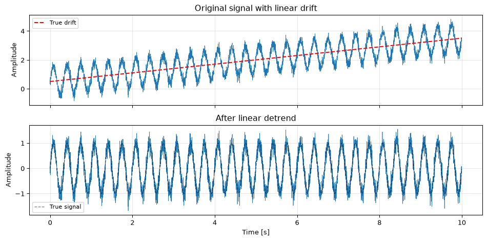
The simplest and most common approach: fit a straight line \(\hat{x}[n] = an + b\) to the signal by least squares and subtract it. This removes any constant offset (DC) and linear drift.
SciPy provides scipy.signal.detrend which does exactly this:
import numpy as npimport matplotlib.pyplot as pltfrom scipy import signal as sigrng = np.random.default_rng(42)fs =500t = np.arange(5000) / fs# Simulated sensor signal: sine + linear drift + noisedrift =0.3* t +0.5x_clean = np.sin(2* np.pi *3* t)x = x_clean + drift +0.2* rng.standard_normal(len(t))x_detrended = sig.detrend(x, type='linear')fig, axes = plt.subplots(2, 1, figsize=(10, 5), sharex=True)axes[0].plot(t, x, 'C0', linewidth=0.5)axes[0].plot(t, drift, 'r--', linewidth=1.5, label='True drift')axes[0].set_title('Original signal with linear drift')axes[0].legend(fontsize=8)axes[0].set_ylabel('Amplitude')axes[1].plot(t, x_detrended, 'C0', linewidth=0.5)axes[1].plot(t, x_clean, 'k--', linewidth=1, alpha=0.5, label='True signal')axes[1].set_title('After linear detrend')axes[1].legend(fontsize=8)axes[1].set_xlabel('Time [s]')axes[1].set_ylabel('Amplitude')for ax in axes: ax.grid(True, alpha=0.3)fig.tight_layout()plt.show()
Figure 1: Linear detrending removes the slow drift, revealing the underlying oscillation.
Linear detrend is fast, robust, and often sufficient. Use type='constant' for DC removal only (subtracts the mean).
Polynomial detrend
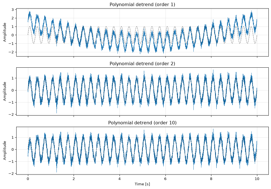
When the drift is not linear (a common situation with thermal effects, sensor aging, or slow environmental changes) you can fit a higher-order polynomial:
\[\hat{x}[n] = \sum_{k=0}^{p} c_k\, n^k\]
and subtract it. NumPy’s polyfit and polyval handle this directly.
Figure 2: Polynomial detrend on a signal with quadratic drift. Order 1 (linear) leaves residual curvature; order 2 (quadratic) matches the drift well; order 10 starts overfitting.
Overfitting
High-order polynomial detrending is tempting but dangerous. A polynomial of order \(p\) has \(p + 1\) free parameters. With high \(p\), the polynomial starts fitting the signal itself, not just the trend. This is especially problematic near the edges of the signal, where polynomial fits tend to oscillate wildly (Runge’s phenomenon). As a rule of thumb, keep \(p \le 5\) unless you have a physical reason for a specific functional form.
High-pass filtering
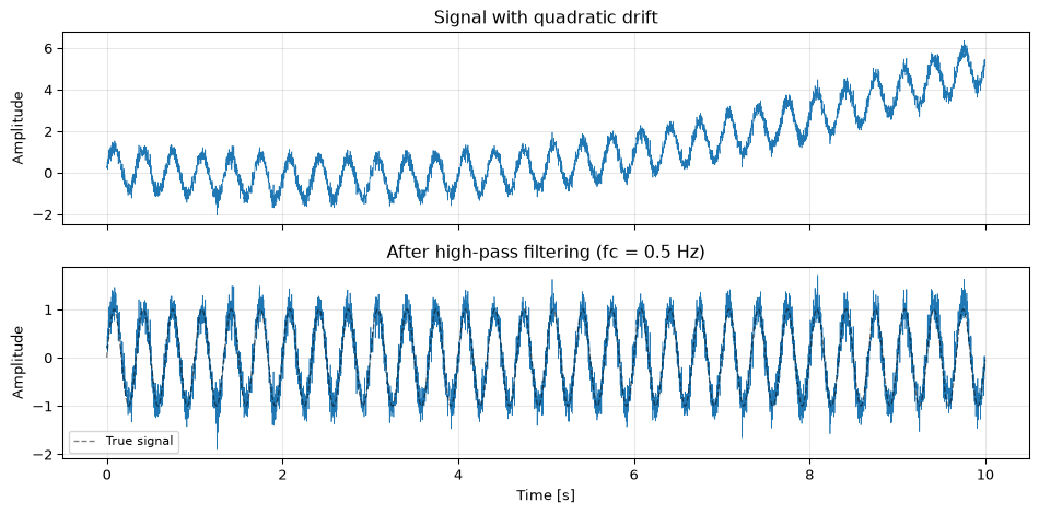
Detrending can also be viewed as a filtering problem: a slow drift is a low-frequency component, so removing it is equivalent to high-pass filtering.
The advantage over polynomial fitting is that high-pass filtering adapts continuously. It does not assume any particular functional form for the trend. The disadvantage is that it also removes legitimate low-frequency signal content, and the transition band means you cannot get a perfectly sharp cutoff between “trend” and “signal.”
Figure 3: High-pass filtering as detrending: a 4th-order Butterworth high-pass at 0.5 Hz removes the slow drift while preserving the 3 Hz signal component.
Note the use of sosfiltfilt (zero-phase filtering) to avoid the phase distortion that a causal filter would introduce. See Zero-phase filtering for details on why this matters.
For real-time applications where you cannot use filtfilt, a causal high-pass filter introduces a transient at the start. The duration of this transient depends on the filter order and cutoff frequency: lower cutoffs mean longer transients.
Savitzky-Golay baseline estimation
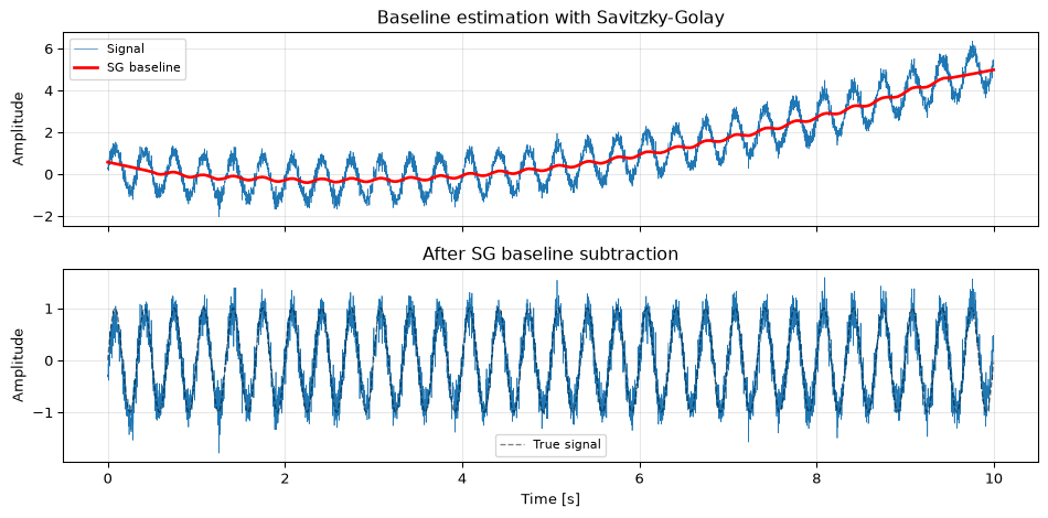
A less common but useful approach: use a Savitzky-Golay filter with a very wide window to estimate the baseline, then subtract it. Because the SG filter preserves low-order polynomial trends by construction, a wide SG window captures the slow drift while ignoring the faster signal components.
Figure 4: Savitzky-Golay baseline estimation: a wide SG window (501 points, order 2) captures the slow drift. Subtracting it yields a clean signal.
The window length must be long enough to span the slowest drift period but not so long that the baseline estimate becomes insensitive to actual trend changes. This method works particularly well for spectroscopy and chromatography data, where peaks sit on a smoothly varying baseline.
Spectral impact of detrending
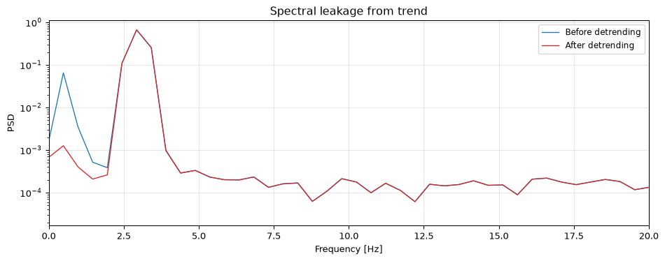
To see why detrending matters for spectral analysis, consider the power spectral density before and after:
Figure 5: PSD before and after detrending. The undetrended signal shows massive low-frequency energy from the drift, masking the 3 Hz signal component. After detrending, the spectral peaks are clearly visible.
Choosing a method
Method
Assumes drift shape?
Real-time?
Handles nonlinear drift?
Watch out for
Linear detrend
Linear
Batch
No
Residual curvature
Polynomial detrend
Polynomial
Batch
Somewhat
Overfitting, edge effects
High-pass filter
None
Yes
Yes
Removes low-freq signal too
SG baseline
Smooth
Batch
Yes
Window length selection
In practice: start with scipy.signal.detrend(x, type='linear'). If there is residual curvature, try a quadratic polynomial or a high-pass filter. Only reach for fancier methods when the simple ones visibly fail.
Open questions
Trend vs signal. The fundamental ambiguity: what is “trend” and what is “signal” is ultimately a modelling decision. A slowly varying physiological signal might be trend in one analysis and the signal of interest in another. No algorithm can resolve this without domain knowledge.
Online detrending. For streaming applications, polynomial detrending requires a buffer and is inherently batch-mode. Recursive least-squares approaches exist for online polynomial fitting but add complexity. A causal high-pass filter is often simpler and good enough, at the cost of a startup transient.
References
Shapley, Robert, and Christina Enroth-Cugell. 1984. “Visual Adaptation and Retinal Gain Controls.”Progress in Retinal Research 3: 263–346.
Source Code
---title: "Detrending"subtitle: "Removing slow drifts from signals"---::: {.callout-tip title="Nature's detrending" appearance="simple"}Your eyes detrend continuously. Retinal photoreceptors adapt to the ambient light level (whether you are in bright sunlight or a dim room) by subtracting the slow-varying background so the visual cortex responds to *changes* in luminance, not absolute brightness [@shapley1984visual]. Without this biological high-pass filter, you would be blinded every time you walked outside.:::Many real-world signals sit on top of slow drifts that have nothing to do with the phenomenon you are measuring. A temperature sensor with thermal drift, an accelerometer with a DC offset that wanders, an ECG signal riding on a baseline that shifts with respiration: in all these cases, the trend obscures the signal of interest and corrupts downstream analysis.Detrending matters for two specific reasons: **stationarity** and **spectral leakage**. Most DSP tools (correlation, spectral analysis, filtering) assume at least weak stationarity. A slow trend violates this assumption and biases results. In the frequency domain, a trend acts like a strong low-frequency component that leaks energy across the spectrum through windowing sidelobes, masking weaker spectral features.::: {.callout-note title="Prerequisites"}This topic assumes familiarity with [frequency-domain analysis](../../basics/05-frequency-domain.qmd) (spectral leakage, windowing) and [filter design](../../basics/06-filter-design.qmd) (high-pass filtering). Background on [noise and SNR](../../basics/03-noise-snr.qmd) is helpful for understanding drift as a noise source.:::---## Linear detrendThe simplest and most common approach: fit a straight line $\hat{x}[n] = an + b$ to the signal by least squares and subtract it. This removes any constant offset (DC) and linear drift.SciPy provides `scipy.signal.detrend` which does exactly this:```{python}#| label: fig-detrend-demo#| fig-cap: "Linear detrending removes the slow drift, revealing the underlying oscillation."import numpy as npimport matplotlib.pyplot as pltfrom scipy import signal as sigrng = np.random.default_rng(42)fs =500t = np.arange(5000) / fs# Simulated sensor signal: sine + linear drift + noisedrift =0.3* t +0.5x_clean = np.sin(2* np.pi *3* t)x = x_clean + drift +0.2* rng.standard_normal(len(t))x_detrended = sig.detrend(x, type='linear')fig, axes = plt.subplots(2, 1, figsize=(10, 5), sharex=True)axes[0].plot(t, x, 'C0', linewidth=0.5)axes[0].plot(t, drift, 'r--', linewidth=1.5, label='True drift')axes[0].set_title('Original signal with linear drift')axes[0].legend(fontsize=8)axes[0].set_ylabel('Amplitude')axes[1].plot(t, x_detrended, 'C0', linewidth=0.5)axes[1].plot(t, x_clean, 'k--', linewidth=1, alpha=0.5, label='True signal')axes[1].set_title('After linear detrend')axes[1].legend(fontsize=8)axes[1].set_xlabel('Time [s]')axes[1].set_ylabel('Amplitude')for ax in axes: ax.grid(True, alpha=0.3)fig.tight_layout()plt.show()```Linear detrend is fast, robust, and often sufficient. Use `type='constant'` for DC removal only (subtracts the mean).---## Polynomial detrendWhen the drift is not linear (a common situation with thermal effects, sensor aging, or slow environmental changes) you can fit a higher-order polynomial:$$\hat{x}[n] = \sum_{k=0}^{p} c_k\, n^k$$and subtract it. NumPy's `polyfit` and `polyval` handle this directly.```{python}#| label: fig-poly-detrend#| fig-cap: "Polynomial detrend on a signal with quadratic drift. Order 1 (linear) leaves residual curvature; order 2 (quadratic) matches the drift well; order 10 starts overfitting."# Quadratic driftdrift_quad =0.1* t**2-0.5* t +0.3x_quad = x_clean + drift_quad +0.2* rng.standard_normal(len(t))fig, axes = plt.subplots(3, 1, figsize=(10, 7), sharex=True)for i, order inenumerate([1, 2, 10]): coeffs = np.polyfit(np.arange(len(x_quad)), x_quad, order) trend = np.polyval(coeffs, np.arange(len(x_quad))) residual = x_quad - trend axes[i].plot(t, residual, 'C0', linewidth=0.5) axes[i].plot(t, x_clean, 'k--', linewidth=1, alpha=0.5) axes[i].set_title(f'Polynomial detrend (order {order})') axes[i].set_ylabel('Amplitude') axes[i].grid(True, alpha=0.3)axes[2].set_xlabel('Time [s]')fig.tight_layout()plt.show()```::: {.callout-warning title="Overfitting"}High-order polynomial detrending is tempting but dangerous. A polynomial of order $p$ has $p + 1$ free parameters. With high $p$, the polynomial starts fitting the signal itself, not just the trend. This is especially problematic near the edges of the signal, where polynomial fits tend to oscillate wildly (Runge's phenomenon). As a rule of thumb, keep $p \le 5$ unless you have a physical reason for a specific functional form.:::---## High-pass filteringDetrending can also be viewed as a filtering problem: a slow drift is a low-frequency component, so removing it is equivalent to high-pass filtering.The advantage over polynomial fitting is that high-pass filtering adapts continuously. It does not assume any particular functional form for the trend. The disadvantage is that it also removes legitimate low-frequency signal content, and the transition band means you cannot get a perfectly sharp cutoff between "trend" and "signal."```{python}#| label: fig-hp-detrend#| fig-cap: "High-pass filtering as detrending: a 4th-order Butterworth high-pass at 0.5 Hz removes the slow drift while preserving the 3 Hz signal component."# High-pass filter at 0.5 Hzsos_hp = sig.butter(4, 0.5, btype='highpass', fs=fs, output='sos')x_hp = sig.sosfiltfilt(sos_hp, x_quad)fig, axes = plt.subplots(2, 1, figsize=(10, 5), sharex=True)axes[0].plot(t, x_quad, 'C0', linewidth=0.5)axes[0].set_title('Signal with quadratic drift')axes[0].set_ylabel('Amplitude')axes[1].plot(t, x_hp, 'C0', linewidth=0.5)axes[1].plot(t, x_clean, 'k--', linewidth=1, alpha=0.5, label='True signal')axes[1].set_title('After high-pass filtering (fc = 0.5 Hz)')axes[1].legend(fontsize=8)axes[1].set_xlabel('Time [s]')axes[1].set_ylabel('Amplitude')for ax in axes: ax.grid(True, alpha=0.3)fig.tight_layout()plt.show()```Note the use of `sosfiltfilt` (zero-phase filtering) to avoid the phase distortion that a causal filter would introduce. See [Zero-phase filtering](../zero-phase/index.qmd) for details on why this matters.For real-time applications where you cannot use `filtfilt`, a causal high-pass filter introduces a transient at the start. The duration of this transient depends on the filter order and cutoff frequency: lower cutoffs mean longer transients.---## Savitzky-Golay baseline estimationA less common but useful approach: use a [Savitzky-Golay filter](../smoothing/index.qmd) with a very wide window to estimate the baseline, then subtract it. Because the SG filter preserves low-order polynomial trends by construction, a wide SG window captures the slow drift while ignoring the faster signal components.```{python}#| label: fig-sg-baseline#| fig-cap: "Savitzky-Golay baseline estimation: a wide SG window (501 points, order 2) captures the slow drift. Subtracting it yields a clean signal."from scipy.signal import savgol_filter# Estimate baseline with a wide SG windowbaseline = savgol_filter(x_quad, window_length=501, polyorder=2)x_sg_detrended = x_quad - baselinefig, axes = plt.subplots(2, 1, figsize=(10, 5), sharex=True)axes[0].plot(t, x_quad, 'C0', linewidth=0.5, label='Signal')axes[0].plot(t, baseline, 'r-', linewidth=2, label='SG baseline')axes[0].set_title('Baseline estimation with Savitzky-Golay')axes[0].legend(fontsize=8)axes[0].set_ylabel('Amplitude')axes[1].plot(t, x_sg_detrended, 'C0', linewidth=0.5)axes[1].plot(t, x_clean, 'k--', linewidth=1, alpha=0.5, label='True signal')axes[1].set_title('After SG baseline subtraction')axes[1].legend(fontsize=8)axes[1].set_xlabel('Time [s]')axes[1].set_ylabel('Amplitude')for ax in axes: ax.grid(True, alpha=0.3)fig.tight_layout()plt.show()```The window length must be long enough to span the slowest drift period but not so long that the baseline estimate becomes insensitive to actual trend changes. This method works particularly well for spectroscopy and chromatography data, where peaks sit on a smoothly varying baseline.---## Spectral impact of detrendingTo see why detrending matters for spectral analysis, consider the power spectral density before and after:```{python}#| label: fig-spectral-impact#| fig-cap: "PSD before and after detrending. The undetrended signal shows massive low-frequency energy from the drift, masking the 3 Hz signal component. After detrending, the spectral peaks are clearly visible."f_raw, P_raw = sig.welch(x_quad, fs, nperseg=1024)f_det, P_det = sig.welch(x_hp, fs, nperseg=1024)fig, ax = plt.subplots(figsize=(10, 4))ax.semilogy(f_raw, P_raw, 'C0', linewidth=1, label='Before detrending')ax.semilogy(f_det, P_det, 'C3', linewidth=1, label='After detrending')ax.set_xlabel('Frequency [Hz]')ax.set_ylabel('PSD')ax.set_xlim(0, 20)ax.legend(fontsize=9)ax.grid(True, alpha=0.3)ax.set_title('Spectral leakage from trend')fig.tight_layout()plt.show()```---## Choosing a method| Method | Assumes drift shape? | Real-time? | Handles nonlinear drift? | Watch out for ||--------|:-:|:-:|:-:|------|| Linear detrend | Linear | Batch | No | Residual curvature || Polynomial detrend | Polynomial | Batch | Somewhat | Overfitting, edge effects || High-pass filter | None | Yes | Yes | Removes low-freq signal too || SG baseline | Smooth | Batch | Yes | Window length selection |**In practice:** start with `scipy.signal.detrend(x, type='linear')`. If there is residual curvature, try a quadratic polynomial or a high-pass filter. Only reach for fancier methods when the simple ones visibly fail.---## Open questions**Trend vs signal.** The fundamental ambiguity: what is "trend" and what is "signal" is ultimately a modelling decision. A slowly varying physiological signal might be trend in one analysis and the signal of interest in another. No algorithm can resolve this without domain knowledge.**Online detrending.** For streaming applications, polynomial detrending requires a buffer and is inherently batch-mode. Recursive least-squares approaches exist for online polynomial fitting but add complexity. A causal high-pass filter is often simpler and good enough, at the cost of a startup transient.