From batch least squares to RLS to the Kalman filter: the same estimate, computed as the data arrives
Every estimator in this arc so far was a batch estimator: collect the whole record, then compute. Real instruments rarely get that luxury. A tone tracker updates while the tone is still sounding, an echo canceller adapts while the far end is still talking, and neither can afford to re-solve a growing least-squares problem from scratch at every sample. The remarkable fact this page builds on is that they do not have to, and that nothing is lost: there is an exact algebraic identity that turns “re-solve the whole problem with one more equation” into “correct the previous answer by its own prediction error”. Followed honestly, that identity walks up a short ladder: batch least squares, recursive least squares, and at the top the Kalman filter, revealed as recursive minimum-mean-square-error estimation rather than the bundle of matrix rituals it is often presented as.
Two neighbouring pages already live on this ladder, and this page deliberately does not repeat them. The adaptive-filtering page owns RLS as an algorithm: its convergence speed against LMS, its \(O(N^2)\) price, its place in the echo-cancelling workhorse rotation. The model-based-filtering page owns the Kalman filter as a practice: state-space models, tracking, tuning, and an embedded implementation. What neither page has is the estimation-theory lineage that connects them to the foundations page and to each other. That lineage is this page’s whole subject, and it ends with the two identities that anchor it, both exact algebra and both pinned by tests: RLS with forgetting factor 1 is batch least squares, and the Kalman filter on a static parameter is recursive weighted least squares.
with \(\mathbf{X}\) a \(k \times p\) design matrix (one regressor row \(\mathbf{x}_i^T\) per observation) and \(\mathbf{n}\) zero-mean noise of variance \(\sigma^2\) per sample. The least-squares estimate solves the normal equations,
which equals the Cramér-Rao bound: the Fisher information of this model is exactly \(\mathbf{J} = \mathbf{X}^T\mathbf{X}/\sigma^2\), so least squares is efficient, not merely convenient. (That closed form is not taken on faith: test_recursive.py builds the Fisher matrix numerically from the log-likelihood curvature and compares.)
The trouble is the record length \(k\): every quantity above silently depends on how many rows \(\mathbf{X}\) has. When observation \(k+1\) arrives, \(\mathbf{X}^T\mathbf{X}\) and \(\mathbf{X}^T\mathbf{y}\) change, and recomputing \(\hat{\boldsymbol{\theta}}\) costs a fresh \(p \times p\) solve, \(O(p^3)\), at every sample, on top of accumulating the products. A 64-tap channel identified at 8 kHz would re-invert a \(64\times 64\) matrix eight thousand times a second. The whole point of the next section is that the inverse at time \(k+1\) is a cheap, exact function of the inverse at time \(k\).
One new equation: the rank-one update
Adding observation \((\mathbf{x}_{k}, y_{k})\) changes the normal equations by the smallest possible amount:
where \(\mathbf{R} = \mathbf{X}^T\mathbf{X}\) and \(\mathbf{r} = \mathbf{X}^T\mathbf{y}\): a rank-one perturbation. The Sherman-Morrison formula (Sherman and Morrison 1950) gives the inverse of a rank-one-perturbed matrix in closed form, with no new inversion:
Write \(\mathbf{P}_k = \mathbf{R}_k^{-1}\), apply the formula with \(\mathbf{u} = \mathbf{v} = \mathbf{x}_k\), define the gain vector\(\mathbf{g}_k\), and three lines of algebra (carried out in full in the thesis quoted below) collapse \(\hat{\boldsymbol{\theta}}_k = \mathbf{P}_k \mathbf{r}_k\) into a recursion that never touches the past data again:
This is recursive least squares. Read the middle two lines slowly, because their shape is the deepest thing on this page: predict the new observation from what you believe, and correct your belief in proportion to how wrong the prediction was. The a priori error \(e_k\) (the innovation) measures surprise; the gain \(\mathbf{g}_k\) decides how much surprise moves the estimate, and it is built from \(\mathbf{P}_k\), which is nothing other than the estimator’s own covariance shape: \(\sigma^2\mathbf{P}_k\) is exactly the batch covariance above. The filter carries its own error bars, and uses them to decide how much to learn. The same predict-and-correct anatomy returns, with a model attached, as the Kalman filter below.
Per update the cost is \(O(p^2)\), with no inversion anywhere, and the result is not an approximation to batch least squares; it is batch least squares, reorganised:
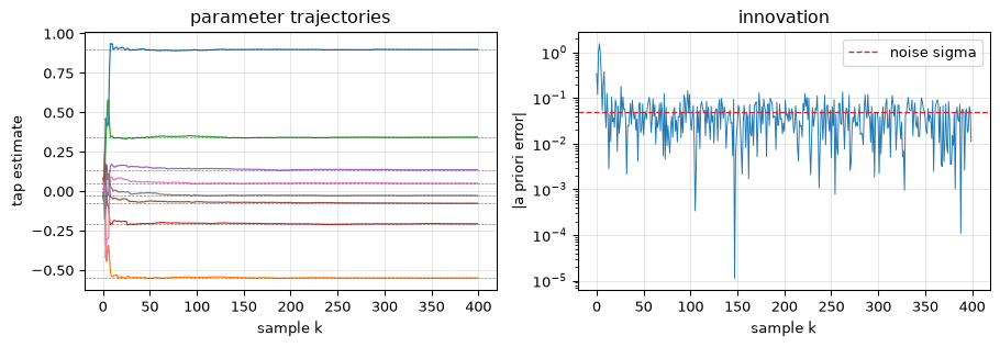
Figure 1: RLS identifying an 8-tap FIR channel from white noise, sample by sample. Left: the eight parameter trajectories lock onto the true taps (dashed) within a few tens of samples. Right: the a priori error collapses to the 0.05 noise floor. After the last sample the recursive estimate and the batch least-squares solution on the same 400 samples agree to better than 1e-9 on every tap: asserted below, not eyeballed.
max |recursive - batch| over all taps: 9.28e-11
From the archive: an MSc thesis, a folder called ‘old shit’, and who wrote what
The primary source for this page is the author’s own MSc thesis (Veen 2001) (TU/e, 2001, supervised by Piet Sommen) and the MATLAB working folder that shipped with it. The thesis is about multichannel acoustic echo cancellation; that subject stays where it is (one honest sentence on it under Going further), and this page quarries only its estimation core: section 5.3 derives exactly the recursion above from the Sherman-Morrison formula, summarises it as “Box 3: Classical RLS-algorithm”, and remarks in passing that it “is a special case of the Kalman filter”, which is the sentence this page grew from.
The code folder is a small archaeology lesson in why version identification comes before verification. It contains three distinct lineages. First, a textbook reference pair, rls.m/rlsinit.m, plainly marked “Copyright 1999 by Todd K. Moon” (companion code to Moon and Stirling (Moon and Stirling 2000)): not the author’s work, and quoted here only for one load-bearing detail, its initialisation convention (next section). (Both live in a subfolder the author labelled “old shit”, which turns out to double as an accurate authorship marker.) Second, working copies of the collaborator’s algorithm family: BRLS2.m through BRLS5.m carry D.W.E. Schobben’s authorship header from his original (preserved in the Daniel/ folder), with the author’s Dutch experiment notes and variant edits layered on top; the algorithms are Schobben’s, the tinkering is the author’s, and nothing from this lineage is used here beyond establishing it. Third, the author’s own unattributed MISO_* scripts, among them MISO_brls.m, which implements the recursion of this page in rank-\(B\) blocks and whose header states its own fixed point: it “calculates the […] left-pseudo inverse closed form solution” iteratively. The batch-equivalence assertion under the figure above is that thirty-year-old header comment, promoted to a machine-checked test.
One reconciliation matters: the Schobben-lineage variants carry a forgetting factor on their correlation estimates, but the recursion the thesis text actually derives (Box 3, and MISO_brls.m with it) has none: it is the growing-window, \(\lambda = 1\) algorithm whose fixed point is batch least squares. Forgetting enters this page two sections down as a deliberate modelling choice, not as an inherited default.
The block form is worth a sentence, because it is the shape the thesis code actually uses: collecting \(B\) new rows \(\mathbf{X}_B\) at a time and applying the matrix-inversion lemma (Sherman-Morrison’s rank-\(B\) generalisation) gives the same fixed point with a \(B \times B\) solve per block. block_rls implements it, and the tests pin \(B = 1\) to the sample recursion and every \(B\) to the batch solution.
A numerical footnote the 2001 code earned the hard way
When \(B > p\), the \(B \times B\) matrix \(\mathbf{I} + \mathbf{X}_B\mathbf{P}\mathbf{X}_B^T\) has \(p\) eigenvalues of order \(\|\mathbf{x}\|^2/\delta\) and \(B - p\) eigenvalues equal to 1, so its condition number is of order \(1/\delta\): enormous, since the initialisation makes \(\delta\) tiny on purpose. Solving the linear system (as block_rls does) shrugs this off; explicitly forming the inverse, as the 2001 MATLAB’s inv() call did, loses most of the difference. With \(\delta = 10^{-10}\) and \(B = 25\) that is the gap between agreeing with batch to about \(10^{-7}\) and to about \(10^{-3}\), measured on this page’s identification problem (on a smaller 4-parameter problem the inv() route was three times worse again). The recursion is exact; the arithmetic is not, and inv() is how you find out.
Initialisation is a prior (and delta is a ridge)
The recursion needs starting values. \(\hat{\boldsymbol{\theta}}_0 = \mathbf{0}\) is natural; \(\mathbf{P}_0\) is not, because the true \(\mathbf{P}\) after zero observations would be the inverse of a zero matrix. The universal fix, and the convention of the thesis code (rlsinit.m reads Prls = 1/delta*eye(m) with delta a small positive constant, and MISO_brls.m uses \(\delta = 10^{-11}\)):
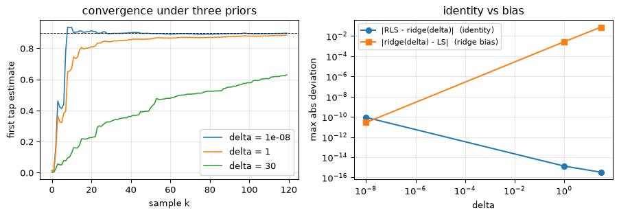
which is ridge regression with ridge weight \(\delta\): the recursion’s starting fiction is precisely a \(\delta\mathbf{I}\) added to the normal-equation matrix. This is an identity, not an approximation, and the tests verify it to 1e-12 for \(\delta\) spanning three orders of magnitude. It also hands \(\delta\) its Bayesian reading: \(\mathbf{P}_0\) is a prior covariance (\(\boldsymbol{\theta} \sim \mathcal{N}(\mathbf{0}, \sigma^2\mathbf{P}_0)\)), small \(\delta\) is a nearly flat prior, and the data overwhelm it at the rate the figure shows.
Show the code
deltas = [1e-8, 1.0, 30.0]fig, axes = plt.subplots(1, 2, figsize=(9.5, 3.4))gaps, biases = [], []for d in deltas: r = RecursiveLeastSquares(p, forgetting=1.0, delta=d) tr = r.fit(X, y) axes[0].plot(tr[:120, 0], lw=1.2, label=f'delta = {d:g}') th_ridge, _ = batch_least_squares(X, y, ridge=d) gaps.append(np.max(np.abs(r.theta - th_ridge))) biases.append(np.max(np.abs(th_ridge - theta_batch)))axes[0].axhline(h_true[0], color='k', ls='--', lw=0.7)axes[0].set_xlabel('sample k'); axes[0].set_ylabel('first tap estimate')axes[0].set_title('convergence under three priors'); axes[0].legend()axes[1].loglog(deltas, gaps, 'o-', label='|RLS - ridge(delta)| (identity)')axes[1].loglog(deltas, biases, 's-', label='|ridge(delta) - LS| (ridge bias)')axes[1].set_xlabel('delta'); axes[1].set_ylabel('max abs deviation')axes[1].set_title('identity vs bias'); axes[1].legend(fontsize=8)for ax in axes: ax.grid(True, alpha=0.3)fig.tight_layout(); plt.show()for d, g inzip(deltas, gaps):print(f"delta = {d:>6g}: max |RLS final - ridge(delta)| = {g:.2e}")assert g <1e-10bias_per_delta = [b / d for b, d inzip(biases, deltas)]print("ridge bias / delta:", ", ".join(f"{r:.5f}"for r in bias_per_delta))assertmax(bias_per_delta) /min(bias_per_delta) <1.5# near-linear in delta
Figure 2: What the initialisation actually does. Left: first-tap trajectory for delta = 1e-8, 1, and 30 on the same data; a large delta (a strong prior pulling toward zero) delays convergence, and moves the destination only by the ridge bias the right panel quantifies. Right: the exact identity behind the picture: at every delta, the final RLS estimate coincides with batch ridge regression using ridge weight delta; the printed maximum deviations stay below 1e-10 (asserted; machine precision for the larger deltas), while the distance to the plain least-squares solution grows linearly with delta (asserted below as a ratio check), which is the ridge bias, not an error.
delta =  1e-08:  max |RLS final - ridge(delta)| = 8.90e-11
delta =      1:  max |RLS final - ridge(delta)| = 1.78e-15
delta =     30:  max |RLS final - ridge(delta)| = 5.55e-16
ridge bias / delta: 0.00274, 0.00273, 0.00250
The parameterisation trap, RLS edition: which way does delta point?
The same failure recurs across these problems: a formula quoted from memory in one convention, applied in another (the sinusoid CRLB’s factor of two, the signed-frequency Fisher sum). RLS initialisation is the recursion’s version of it. The literature writes both \(\mathbf{P}_0 = \delta^{-1}\mathbf{I}\) with \(\delta\)small (the thesis code’s convention, used throughout this page) and \(\mathbf{P}_0 = \delta\mathbf{I}\) with \(\delta\)large: same filter, same letter, opposite roles. Quoting a recipe like “initialise with delta = 0.01” across the convention boundary silently changes the prior by four orders of magnitude. The disambiguation is physical, not typographic: \(\mathbf{P}_0\) itself must be large for a weak prior, and the ridge identity above gives the scalar its units: whatever symbol it wears, the number added to every eigenvalue of \(\mathbf{X}^T\mathbf{X}\) is \(1/\lVert\mathbf{P}_0\rVert\). Before quoting any RLS pseudocode, run it at \(\lambda = 1\) against a batch solve; the check costs five lines (the test suite here does exactly that) and settles the convention question unambiguously.
Forgetting: the price of tracking a moving world
Everything so far assumed \(\boldsymbol{\theta}\) never changes, and the recursion honours that: as \(k \to \infty\), \(\mathbf{P}_k \to \mathbf{0}\), the gain dies, and the filter stops listening: correct behaviour for a constant, fatal for a drifting one. The standard repair discounts old data exponentially, minimising \(\sum_i \lambda^{k-i} e_i^2\) with a forgetting factor\(0 < \lambda \le 1\), which edits the recursion in exactly two places:
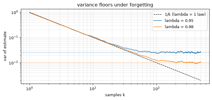
The adaptive-filtering page uses this daily; what belongs here is its estimation-theoretic price tag. A filter that forgets is no longer consistent. For the cleanest case, estimating a constant scalar in white noise (regressor \(x = 1\)), the estimate becomes an exponentially weighted mean with normalised weights \((1-\lambda)\lambda^j\), and its steady-state variance is
At \(\lambda = 1\) the variance falls as \(\sigma^2/k\) forever, the foundations page’s\(\sqrt{N}\) law; at \(\lambda < 1\) it stops falling at a floor. Forgetting spends statistical efficiency to buy the ability to notice change; the covariance floor is the receipt, an honest record of how much certainty the filter declined to accumulate.
Figure 3: The price of forgetting, measured. Monte Carlo variance (1000 runs) of the RLS estimate of a constant in unit-variance noise. At lambda = 1 the variance tracks 1/k indefinitely. At lambda = 0.95 and 0.98 it leaves the 1/k line (dashed) and flattens onto the predicted floor (1-lambda)/(1+lambda) (dotted, one per lambda); the measured floors land within a few percent of the closed form, and the assertion below checks the ratio, not just the two operands.
Two ‘effective windows’, a factor of two apart
“\(\lambda = 0.98\) is like averaging the last \(N\) samples”: true, but which \(N\)? The weights sum to \(1/(1-\lambda)\), giving the widely quoted weight-sum window\(N_w = 50\). But a plain mean with the same variance as the exponentially weighted one needs, by the floor formula above,
\[N_{\mathrm{var}} = \frac{1+\lambda}{1-\lambda} = 99 \text{ samples at } \lambda = 0.98 \quad \Bigl(\approx \frac{2}{1-\lambda}, \text{ the rough count, here } 100\Bigr):\]
twice as many. Both conventions are in circulation, usually without a subscript, and any noise-floor or CRLB comparison that borrows the wrong one is silently optimistic or pessimistic by 3 dB. The test suite asserts the relationship (\(N_{\mathrm{var}}/N_w = 1 + \lambda\), hence the factor two in the limit) rather than either number alone.
The Kalman filter is this recursion, given a model
Two upgrades separate RLS from the Kalman filter, and both are already latent in the algebra.
Upgrade one: per-sample trust. Let each observation carry its own noise variance \(r_k\), and weight it accordingly, which the gain absorbs without ceremony:
Fisher information adding, one observation’s worth at a time, exactly the additivity the foundations page proved for independent samples. The recursion is bookkeeping for an information ledger.
Upgrade two: let the parameter move, on purpose. Forgetting handled drift by discounting the past blindly. The principled version writes a model for how the parameter moves: a random walk \(\boldsymbol{\theta}_k = \boldsymbol{\theta}_{k-1} + \mathbf{w}_k\) with \(\operatorname{cov}(\mathbf{w}_k) = q\,\mathbf{I}\), observed through \(y_k = \mathbf{x}_k^T\boldsymbol{\theta}_k + v_k\). Then between observations the estimate stays put (the walk has zero mean) but the uncertainty grows,
and the update runs exactly as before on the inflated covariance. Predict, then correct; uncertainty opens, information closes it. That two-step is the Kalman filter (Kalman 1960), here in the special dress \(\mathbf{F} = \mathbf{I}\) (the model-based-filtering page wears the general one, where states have dynamics like velocity and the same machinery tracks a moving truck). And its optimality claim is the arc’s own criterion: for the linear-Gaussian model the filter computes the conditional mean of the state given all data so far, which is the minimum-mean-square-error estimate; the “gain times innovation” correction is not a heuristic but the Bayesian posterior update, weighting prior against measurement by their inverse variances. In the scalar case (writing plain \(P\) for the now-scalar variance, not the tap count \(p\) of the figures) the gain is simply \(K = P/(P + r)\): believe the measurement in proportion to how uncertain you were.
The claims in this ladder are all exact, and all tested:
\(q = 0\), equal \(r\): the Kalman filter reproduces the RLS trajectories of the first figure at every sample (asserted to 1e-9).
\(q = 0\), per-sample \(r_k\): it reproduces batch weighted least squares, the page’s second anchor identity.
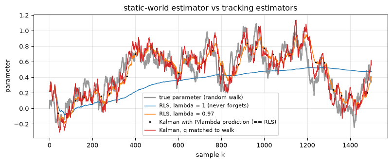
Forgetting is a crude \(q\): the prediction \(\mathbf{P} \leftarrow \mathbf{P}/\lambda\) equals \(\mathbf{P} \leftarrow \mathbf{P} + \mathbf{Q}\) with \(\mathbf{Q} = (\tfrac{1}{\lambda} - 1)\mathbf{P}\), a process noise proportional to the current covariance. Run both; the trajectories coincide exactly. So RLS-with-forgetting is a Kalman filter whose model assumes the parameter wanders more when you know it less, a strange physics, which is why a measured \(q\) beats a tuned \(\lambda\) when you actually know the drift rate.
With \(q > 0\) the covariance no longer collapses: the scalar steady state solves \(P^2 + Pq - qr = 0\), giving \(P_\infty = \bigl(\sqrt{q^2 + 4qr} - q\bigr)/2\), the one-line Riccati equation (tested against the filter’s long run).
Figure 4: Tracking a drifting parameter (grey: truth, a random walk observed in noise). The lambda = 1 filter (blue) is the batch estimator in disguise: it averages the parameter’s entire history and lags ever further behind. RLS with lambda = 0.97 (orange) tracks; the Kalman filter whose process noise q matches the true walk variance (red) tracks as well and is the MMSE estimator by construction. The overlaid dots verify the exact correspondence claim: a Kalman filter run with the P/lambda prediction reproduces the RLS trajectory sample for sample (asserted below 1e-8; the measured gap is printed).
The model-based-filtering page picks the story up from here: real state vectors (\(\mathbf{F} \ne \mathbf{I}\), states the sensor never observes directly), tuning \(\mathbf{Q}\) and \(\mathbf{R}\) honestly, divergence when the model lies, and an embedded implementation on the default platforms. This page deliberately has no embedded companion: the metal for its recursion already exists there. For RLS on hardware, the adaptive-filtering page prices the family honestly (\(O(N^2)\) per sample, divergence risk), its embedded companion shows why NLMS rather than RLS is what usually ships on small metal, and the square-root note under Going further below is the numerical survival kit.
When least squares lies: noise in the regressors
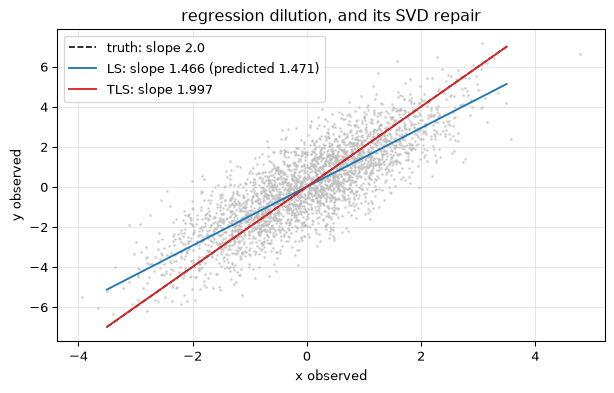
One assumption has ridden along unexamined since the first equation: the design matrix \(\mathbf{X}\) is exact. Noise lives in \(\mathbf{y}\) only. For a curve fit against a clean time axis that is true; for system identification it often is not, because the “input” was measured by an instrument too. And the failure mode is not extra variance but bias that no amount of data cures. For the scalar case \(y = a\,x_{\mathrm{true}} + n\) observed through \(x = x_{\mathrm{true}} + u\),
the attenuation (regression dilution) factor: the noisy regressor inflates the denominator \(\sum x^2\) while the noise averages out of the numerator. The estimator converges, confidently, to the wrong answer.
Total least squares(Golub and Van Loan 1980) repairs the model instead of the symptom: it seeks the smallest joint perturbation of \([\mathbf{X}\;\mathbf{y}]\) making the system consistent, equivalently an orthogonal regression, and the solution drops out of the SVD: take the right singular vector \(\mathbf{v}\) of \([\mathbf{X}\;\mathbf{y}]\) belonging to the smallest singular value, rescale it so its last entry is \(-1\), and its first \(p\) entries are \(\hat{\boldsymbol{\theta}}_{\mathrm{TLS}}\). Its honesty clause: “smallest joint perturbation” presumes the errors in \(\mathbf{X}\) and \(\mathbf{y}\) share one variance; with unequal known variances, scale columns first, and with unknown ratios TLS inherits a convention trap of its own.
Figure 5: Errors in variables, and the two fits. The data (grey) are y = 2x with noise of equal variance in BOTH coordinates (sigma = 0.6 on each, against unit signal variance). Ordinary LS (blue) converges to the attenuated slope 2 x 1/(1+0.36) = 1.47, and its 200 000 samples make it precisely, repeatably wrong; the measured ratio slope/2 matches the closed-form kappa to 1% (asserted). TLS via the SVD (red) treats both coordinates as noisy and recovers the true slope within 1%.
LS slope ratio 0.7331 vs kappa 0.7353; TLS slope 1.9975
From the archive: an errors-in-variables criterion, four noise models deep
One of the author’s research-era notes applies exactly this idea to two-channel frequency-domain system identification: channel 1 measures an unknown source spectrum \(S(f)\) in noise, channel 2 measures the same source through a parametric channel \(G(f) = e^{-\gamma(f) d}\) in more noise, and both channels are noisy, so LS against channel 1 dilutes just like the figure above. The note eliminates the nuisance spectrum \(S(f)\) analytically and lands on the concentrated criterion
worked through four progressively harder noise models (white and equal, white and unequal, colored, correlated-and-colored, the last twice, the second time in matrix notation). All four closed forms are checked by direct numerical minimisation over \(S(f)\) (fd_tls_criterion and its tests), and the denominator is the whole story: LS would divide by \(P_{N_2}\) alone, and the extra \(P_{N_1}\lvert G\rvert^2\) is precisely the reference channel’s noise refusing to be ignored. With \(G = e^{-j2\pi f d}\) this \(J\) is a TLS-flavoured cousin of the time-delay estimators of the previous page, and one test recovers a delay by minimising it.
Two honesty notes about the source. Its Gaussian densities carry a real-variable habit, \(\exp(-\lvert N\rvert^2/2P_N)\) where a proper complex variable wants \(\exp(-\lvert N\rvert^2/P_N)\) (the per-bin complex density on the periodogram page is the correct form); here it is harmless, since a positive constant in the exponent moves no minimiser. And the matrix-notation section ends mid-thought, in Dutch: “Deze uitdrukking moet veel verder te vereenvoudigen zijn” (“this expression should simplify much further”). It should. It is left as it was found: an open question, honestly recorded.
A sibling derivation, “Constrained least-squares polynomial fitting”, handles the opposite situation: the model is trusted more than the data, some points exactly (a fit forced through known values via Lagrange multipliers). Its two-inverse closed form is implemented and tested as constrained_least_squares.
Going further
Square roots against roundoff. The \(\mathbf{P}\) recursion subtracts, and subtraction is where positive-definiteness quietly dies in single precision on long runs. Square-root and UDU\(^T\) filters propagate a factor of \(\mathbf{P}\) instead, guaranteeing \(\mathbf{P} \succ 0\) by construction (Anderson and Moore 1979); the same concern already surfaced as this page’s inv()-versus-solve footnote, and it is the first thing to reach for when an embedded RLS misbehaves after minutes of runtime.
Fast RLS and lattices. The \(O(p^2)\) per sample can be beaten when the regressor is a tapped delay line: fast transversal and lattice RLS reach \(O(p)\) by exploiting the shift structure (Haykin 2002), at a notorious price in numerical fragility.
Rank deficiency, the thesis’s real subject. When multiple input channels are correlated (a stereo far end driving one echo path), \(\mathbf{X}^T\mathbf{X}\) is rank deficient, the solution is not unique, and the recursion of this page converges to the minimum-norm member of the solution set: recursion does not rescue identifiability, it just picks an answer politely. That fact, and what to do about it in multichannel acoustic echo cancellation, is what the source thesis (Veen 2001) is actually about, and it stays a pointer here.
The exponential family beyond Gaussians. Recursive MMSE for linear-Gaussian models is exact; for anything else (nonlinear measurements, non-Gaussian noise) the conditional mean stops being linear in the data, and the extended/unscented approximations and particle filters of the model-based-filtering page’s closing notes take over.
References
Anderson, Brian D. O., and John B. Moore. 1979. Optimal Filtering. Prentice-Hall.
Golub, Gene H., and Charles F. Van Loan. 1980. “An Analysis of the Total Least Squares Problem.”SIAM Journal on Numerical Analysis 17 (6): 883–93.
Kalman, Rudolf E. 1960. “A New Approach to Linear Filtering and Prediction Problems.”Journal of Basic Engineering 82 (1): 35–45. https://doi.org/10.1115/1.3662552.
Moon, Todd K., and Wynn C. Stirling. 2000. Mathematical Methods and Algorithms for Signal Processing. Prentice Hall.
Sherman, Jack, and Winifred J. Morrison. 1950. “Adjustment of an Inverse Matrix Corresponding to a Change in One Element of a Given Matrix.”The Annals of Mathematical Statistics 21 (1): 124–27.
Veen, Jeroen. 2001. “Multi-Channel Acoustic Echo Cancellation.” Master’s thesis, Eindhoven University of Technology, Signal Processing Systems group.
Source Code
---title: "Recursive Estimation"subtitle: "From batch least squares to RLS to the Kalman filter: the same estimate, computed as the data arrives"description-meta: "From batch least squares to RLS to the Kalman filter: the same estimate, computed as the data arrives instead of after it."bibliography: ../../references.bib---Every estimator in this arc so far was a *batch* estimator: collect the whole record, then compute. Real instruments rarely get that luxury. A tone tracker updates while the tone is still sounding, an echo canceller adapts while the far end is still talking, and neither can afford to re-solve a growing least-squares problem from scratch at every sample. The remarkable fact this page builds on is that they do not have to, and that nothing is lost: there is an exact algebraic identity that turns "re-solve the whole problem with one more equation" into "correct the previous answer by its own prediction error". Followed honestly, that identity walks up a short ladder: batch least squares, recursive least squares, and at the top the Kalman filter, revealed as recursive minimum-mean-square-error estimation rather than the bundle of matrix rituals it is often presented as.Two neighbouring pages already live on this ladder, and this page deliberately does not repeat them. The [adaptive-filtering page](../adaptive-filtering/index.qmd) owns RLS *as an algorithm*: its convergence speed against LMS, its $O(N^2)$ price, its place in the echo-cancelling workhorse rotation. The [model-based-filtering page](../model-based-filtering/index.qmd) owns the Kalman filter *as a practice*: state-space models, tracking, tuning, and an embedded implementation. What neither page has is the estimation-theory lineage that connects them to the [foundations page](../estimation-basics/index.qmd) and to each other. That lineage is this page's whole subject, and it ends with the two identities that anchor it, both exact algebra and both pinned by tests: RLS with forgetting factor 1 *is* batch least squares, and the Kalman filter on a static parameter *is* recursive weighted least squares.::: {.callout-note title="Prerequisites"}Part of the [estimation & detection arc](../estimation-and-detection.qmd); the overview gives the reading order.[Estimation basics](../estimation-basics/index.qmd) supplies least squares, Fisher information, and the CRLB; [adaptive filtering](../adaptive-filtering/index.qmd) is where RLS earns its living; [model-based filtering](../model-based-filtering/index.qmd) is where the Kalman filter does.:::::: {.callout-tip title="Code"}The implementation is [`recursive.py`](recursive.py). Save [`test_recursive.py`](test_recursive.py) beside it and `pytest test_recursive.py` runs the checks on it.:::```{python}#| echo: falseimport numpy as npimport matplotlib.pyplot as pltfrom recursive import (attenuation_factor, batch_least_squares, block_rls, constrained_least_squares, ew_variance_factor, fd_tls_criterion, kalman_parameter_filter, RecursiveLeastSquares, total_least_squares, variance_equivalent_window)```<hr>## The batch baseline, and its growing billThe linear model that carried the [weighted-least-squares section](../estimation-basics/index.qmd#prior-knowledge-beats-more-data-weighted-least-squares) of the foundations page:$$\mathbf{y} = \mathbf{X}\boldsymbol{\theta} + \mathbf{n},$$with $\mathbf{X}$ a $k \times p$ design matrix (one regressor row $\mathbf{x}_i^T$ per observation) and $\mathbf{n}$ zero-mean noise of variance $\sigma^2$ per sample. The least-squares estimate solves the normal equations,$$\hat{\boldsymbol{\theta}} = (\mathbf{X}^T\mathbf{X})^{-1}\mathbf{X}^T\mathbf{y},$$and for white Gaussian noise it is also the maximum-likelihood estimate, is unbiased, and has covariance$$\operatorname{cov}(\hat{\boldsymbol{\theta}}) = \sigma^2 (\mathbf{X}^T\mathbf{X})^{-1},$$which equals the Cramér-Rao bound: the Fisher information of this model is exactly $\mathbf{J} = \mathbf{X}^T\mathbf{X}/\sigma^2$, so least squares is efficient, not merely convenient. (That closed form is not taken on faith: `test_recursive.py` builds the Fisher matrix numerically from the log-likelihood curvature and compares.)The trouble is the record length $k$: every quantity above silently depends on how many rows $\mathbf{X}$ has. When observation $k+1$ arrives, $\mathbf{X}^T\mathbf{X}$ and $\mathbf{X}^T\mathbf{y}$ change, and recomputing $\hat{\boldsymbol{\theta}}$ costs a fresh $p \times p$ solve, $O(p^3)$, at *every* sample, on top of accumulating the products. A 64-tap channel identified at 8 kHz would re-invert a $64\times 64$ matrix eight thousand times a second. The whole point of the next section is that the inverse at time $k+1$ is a cheap, exact function of the inverse at time $k$.<hr>## One new equation: the rank-one updateAdding observation $(\mathbf{x}_{k}, y_{k})$ changes the normal equations by the smallest possible amount:$$\mathbf{R}_k = \mathbf{R}_{k-1} + \mathbf{x}_k\mathbf{x}_k^T, \qquad \mathbf{r}_k = \mathbf{r}_{k-1} + \mathbf{x}_k y_k,$$where $\mathbf{R} = \mathbf{X}^T\mathbf{X}$ and $\mathbf{r} = \mathbf{X}^T\mathbf{y}$: a rank-one perturbation. The Sherman-Morrison formula [@sherman1950adjustment] gives the inverse of a rank-one-perturbed matrix in closed form, with no new inversion:$$(\mathbf{A} + \mathbf{u}\mathbf{v}^T)^{-1} = \mathbf{A}^{-1} - \frac{\mathbf{A}^{-1}\mathbf{u}\mathbf{v}^T\mathbf{A}^{-1}}{1 + \mathbf{v}^T\mathbf{A}^{-1}\mathbf{u}}.$$Write $\mathbf{P}_k = \mathbf{R}_k^{-1}$, apply the formula with $\mathbf{u} = \mathbf{v} = \mathbf{x}_k$, define the **gain vector** $\mathbf{g}_k$, and three lines of algebra (carried out in full in the thesis quoted below) collapse $\hat{\boldsymbol{\theta}}_k = \mathbf{P}_k \mathbf{r}_k$ into a recursion that never touches the past data again:$$\mathbf{g}_k = \frac{\mathbf{P}_{k-1}\mathbf{x}_k}{1 + \mathbf{x}_k^T\mathbf{P}_{k-1}\mathbf{x}_k},$$$$e_k = y_k - \mathbf{x}_k^T\hat{\boldsymbol{\theta}}_{k-1},$$$$\hat{\boldsymbol{\theta}}_k = \hat{\boldsymbol{\theta}}_{k-1} + \mathbf{g}_k\, e_k,$$$$\mathbf{P}_k = \mathbf{P}_{k-1} - \mathbf{g}_k\mathbf{x}_k^T\mathbf{P}_{k-1}.$$This is **recursive least squares**. Read the middle two lines slowly, because their shape is the deepest thing on this page: *predict the new observation from what you believe, and correct your belief in proportion to how wrong the prediction was*. The a priori error $e_k$ (the **innovation**) measures surprise; the gain $\mathbf{g}_k$ decides how much surprise moves the estimate, and it is built from $\mathbf{P}_k$, which is nothing other than the estimator's own covariance shape: $\sigma^2\mathbf{P}_k$ is exactly the batch covariance above. The filter carries its own error bars, and uses them to decide how much to learn. The same predict-and-correct anatomy returns, with a model attached, as the Kalman filter below.Per update the cost is $O(p^2)$, with no inversion anywhere, and the result is not an approximation to batch least squares; it *is* batch least squares, reorganised:```{python}#| label: fig-rls-converges#| fig-cap: "RLS identifying an 8-tap FIR channel from white noise, sample by sample. Left: the eight parameter trajectories lock onto the true taps (dashed) within a few tens of samples. Right: the a priori error collapses to the 0.05 noise floor. After the last sample the recursive estimate and the batch least-squares solution on the same 400 samples agree to better than 1e-9 on every tap: asserted below, not eyeballed."rng = np.random.default_rng(42)p, n =8, 400h_true = np.array([0.9, -0.55, 0.34, -0.21, 0.13, -0.08, 0.05, -0.03])u = rng.normal(size=n + p -1)X = np.array([u[i:i + p][::-1] for i inrange(n)])y = X @ h_true +0.05* rng.normal(size=n)rls = RecursiveLeastSquares(p, forgetting=1.0, delta=1e-8)traj = np.empty((n, p))err = np.empty(n)for k inrange(n): err[k] = rls.update(X[k], y[k]) traj[k] = rls.thetatheta_batch, _ = batch_least_squares(X, y)gap = np.max(np.abs(rls.theta - theta_batch))fig, axes = plt.subplots(1, 2, figsize=(9.5, 3.4))for j inrange(p): axes[0].plot(traj[:, j], lw=0.9) axes[0].axhline(h_true[j], color='k', ls='--', lw=0.5, alpha=0.5)axes[0].set_xlabel('sample k'); axes[0].set_ylabel('tap estimate')axes[0].set_title('parameter trajectories')axes[1].semilogy(np.abs(err) +1e-12, lw=0.7)axes[1].axhline(0.05, color='C3', ls='--', lw=1, label='noise sigma')axes[1].set_xlabel('sample k'); axes[1].set_ylabel('|a priori error|')axes[1].set_title('innovation'); axes[1].legend()for ax in axes: ax.grid(True, alpha=0.3)fig.tight_layout(); plt.show()print(f"max |recursive - batch| over all taps: {gap:.2e}")assert gap <1e-9```::: {.callout-note title="From the archive: an MSc thesis, a folder called 'old shit', and who wrote what"}The primary source for this page is the author's own MSc thesis [@veen2001mcaec] (TU/e, 2001, supervised by Piet Sommen) and the MATLAB working folder that shipped with it. The thesis is about multichannel acoustic echo cancellation; that subject stays where it is (one honest sentence on it under Going further), and this page quarries only its estimation core: section 5.3 derives exactly the recursion above from the Sherman-Morrison formula, summarises it as "Box 3: Classical RLS-algorithm", and remarks in passing that it "is a special case of the Kalman filter", which is the sentence this page grew from.The code folder is a small archaeology lesson in why *version identification comes before verification*. It contains three distinct lineages. First, a textbook reference pair, `rls.m`/`rlsinit.m`, plainly marked "Copyright 1999 by Todd K. Moon" (companion code to Moon and Stirling [@moon2000mathematical]): not the author's work, and quoted here only for one load-bearing detail, its initialisation convention (next section). (Both live in a subfolder the author labelled "old shit", which turns out to double as an accurate authorship marker.) Second, working copies of the collaborator's algorithm family: `BRLS2.m` through `BRLS5.m` carry D.W.E. Schobben's authorship header from his original (preserved in the `Daniel/` folder), with the author's Dutch experiment notes and variant edits layered on top; the algorithms are Schobben's, the tinkering is the author's, and nothing from this lineage is used here beyond establishing it. Third, the author's own unattributed `MISO_*` scripts, among them `MISO_brls.m`, which implements the recursion of this page in rank-$B$ blocks and whose header states its own fixed point: it "calculates the [...] left-pseudo inverse closed form solution" iteratively. The batch-equivalence assertion under the figure above is that thirty-year-old header comment, promoted to a machine-checked test.One reconciliation matters: the Schobben-lineage variants carry a forgetting factor on their correlation estimates, but the recursion the thesis text actually derives (Box 3, and `MISO_brls.m` with it) has *none*: it is the growing-window, $\lambda = 1$ algorithm whose fixed point is batch least squares. Forgetting enters this page two sections down as a deliberate modelling choice, not as an inherited default.:::The block form is worth a sentence, because it is the shape the thesis code actually uses: collecting $B$ new rows $\mathbf{X}_B$ at a time and applying the matrix-inversion lemma (Sherman-Morrison's rank-$B$ generalisation) gives the same fixed point with a $B \times B$ solve per block. `block_rls` implements it, and the tests pin $B = 1$ to the sample recursion and every $B$ to the batch solution.::: {.callout-warning title="A numerical footnote the 2001 code earned the hard way"}When $B > p$, the $B \times B$ matrix $\mathbf{I} + \mathbf{X}_B\mathbf{P}\mathbf{X}_B^T$ has $p$ eigenvalues of order $\|\mathbf{x}\|^2/\delta$ and $B - p$ eigenvalues equal to 1, so its condition number is of order $1/\delta$: enormous, since the initialisation makes $\delta$ tiny on purpose. Solving the linear system (as `block_rls` does) shrugs this off; explicitly forming the inverse, as the 2001 MATLAB's `inv()` call did, loses most of the difference. With $\delta = 10^{-10}$ and $B = 25$ that is the gap between agreeing with batch to about $10^{-7}$ and to about $10^{-3}$, measured on this page's identification problem (on a smaller 4-parameter problem the `inv()` route was three times worse again). The recursion is exact; the arithmetic is not, and `inv()` is how you find out.:::<hr>## Initialisation is a prior (and delta is a ridge)The recursion needs starting values. $\hat{\boldsymbol{\theta}}_0 = \mathbf{0}$ is natural; $\mathbf{P}_0$ is not, because the true $\mathbf{P}$ after zero observations would be the inverse of a zero matrix. The universal fix, and the convention of the thesis code (`rlsinit.m` reads `Prls = 1/delta*eye(m)` with `delta` a small positive constant, and `MISO_brls.m` uses $\delta = 10^{-11}$):$$\mathbf{P}_0 = \frac{1}{\delta}\,\mathbf{I}, \qquad \delta \text{ small}.$$What does that choice *mean*? Unwind the recursion: at $\lambda = 1$ it maintains, exactly,$$\mathbf{P}_k = \Bigl(\delta\mathbf{I} + \textstyle\sum_{i \le k} \mathbf{x}_i\mathbf{x}_i^T\Bigr)^{-1},\qquad\hat{\boldsymbol{\theta}}_k = \mathbf{P}_k \textstyle\sum_{i \le k} \mathbf{x}_i y_i,$$which is **ridge regression** with ridge weight $\delta$: the recursion's starting fiction is precisely a $\delta\mathbf{I}$ added to the normal-equation matrix. This is an identity, not an approximation, and the tests verify it to 1e-12 for $\delta$ spanning three orders of magnitude. It also hands $\delta$ its Bayesian reading: $\mathbf{P}_0$ is a prior covariance ($\boldsymbol{\theta} \sim \mathcal{N}(\mathbf{0}, \sigma^2\mathbf{P}_0)$), small $\delta$ is a nearly flat prior, and the data overwhelm it at the rate the figure shows.```{python}#| label: fig-delta-ridge#| fig-cap: "What the initialisation actually does. Left: first-tap trajectory for delta = 1e-8, 1, and 30 on the same data; a large delta (a strong prior pulling toward zero) delays convergence, and moves the destination only by the ridge bias the right panel quantifies. Right: the exact identity behind the picture: at every delta, the final RLS estimate coincides with batch ridge regression using ridge weight delta; the printed maximum deviations stay below 1e-10 (asserted; machine precision for the larger deltas), while the distance to the plain least-squares solution grows linearly with delta (asserted below as a ratio check), which is the ridge bias, not an error."deltas = [1e-8, 1.0, 30.0]fig, axes = plt.subplots(1, 2, figsize=(9.5, 3.4))gaps, biases = [], []for d in deltas: r = RecursiveLeastSquares(p, forgetting=1.0, delta=d) tr = r.fit(X, y) axes[0].plot(tr[:120, 0], lw=1.2, label=f'delta = {d:g}') th_ridge, _ = batch_least_squares(X, y, ridge=d) gaps.append(np.max(np.abs(r.theta - th_ridge))) biases.append(np.max(np.abs(th_ridge - theta_batch)))axes[0].axhline(h_true[0], color='k', ls='--', lw=0.7)axes[0].set_xlabel('sample k'); axes[0].set_ylabel('first tap estimate')axes[0].set_title('convergence under three priors'); axes[0].legend()axes[1].loglog(deltas, gaps, 'o-', label='|RLS - ridge(delta)| (identity)')axes[1].loglog(deltas, biases, 's-', label='|ridge(delta) - LS| (ridge bias)')axes[1].set_xlabel('delta'); axes[1].set_ylabel('max abs deviation')axes[1].set_title('identity vs bias'); axes[1].legend(fontsize=8)for ax in axes: ax.grid(True, alpha=0.3)fig.tight_layout(); plt.show()for d, g inzip(deltas, gaps):print(f"delta = {d:>6g}: max |RLS final - ridge(delta)| = {g:.2e}")assert g <1e-10bias_per_delta = [b / d for b, d inzip(biases, deltas)]print("ridge bias / delta:", ", ".join(f"{r:.5f}"for r in bias_per_delta))assertmax(bias_per_delta) /min(bias_per_delta) <1.5# near-linear in delta```::: {.callout-warning title="The parameterisation trap, RLS edition: which way does delta point?"}The same failure recurs across these problems: a formula quoted from memory in one convention, applied in another ([the sinusoid CRLB's factor of two](../estimating-a-sinusoid/index.qmd), [the signed-frequency Fisher sum](../time-delay-estimation/index.qmd)). RLS initialisation is the recursion's version of it. The literature writes both $\mathbf{P}_0 = \delta^{-1}\mathbf{I}$ with $\delta$ *small* (the thesis code's convention, used throughout this page) and $\mathbf{P}_0 = \delta\mathbf{I}$ with $\delta$ *large*: same filter, same letter, opposite roles. Quoting a recipe like "initialise with delta = 0.01" across the convention boundary silently changes the prior by four orders of magnitude. The disambiguation is physical, not typographic: $\mathbf{P}_0$ itself must be **large** for a weak prior, and the ridge identity above gives the scalar its units: whatever symbol it wears, the number added to every eigenvalue of $\mathbf{X}^T\mathbf{X}$ is $1/\lVert\mathbf{P}_0\rVert$. Before quoting any RLS pseudocode, run it at $\lambda = 1$ against a batch solve; the check costs five lines (the test suite here does exactly that) and settles the convention question unambiguously.:::<hr>## Forgetting: the price of tracking a moving worldEverything so far assumed $\boldsymbol{\theta}$ never changes, and the recursion honours that: as $k \to \infty$, $\mathbf{P}_k \to \mathbf{0}$, the gain dies, and the filter stops listening: correct behaviour for a constant, fatal for a drifting one. The standard repair discounts old data exponentially, minimising $\sum_i \lambda^{k-i} e_i^2$ with a **forgetting factor** $0 < \lambda \le 1$, which edits the recursion in exactly two places:$$\mathbf{g}_k = \frac{\mathbf{P}_{k-1}\mathbf{x}_k}{\lambda + \mathbf{x}_k^T\mathbf{P}_{k-1}\mathbf{x}_k},\qquad\mathbf{P}_k = \frac{1}{\lambda}\bigl(\mathbf{P}_{k-1} - \mathbf{g}_k\mathbf{x}_k^T\mathbf{P}_{k-1}\bigr).$$The [adaptive-filtering page](../adaptive-filtering/index.qmd#rls-recursive-least-squares) uses this daily; what belongs *here* is its estimation-theoretic price tag. A filter that forgets is no longer consistent. For the cleanest case, estimating a constant scalar in white noise (regressor $x = 1$), the estimate becomes an exponentially weighted mean with normalised weights $(1-\lambda)\lambda^j$, and its steady-state variance is$$\operatorname{var}(\hat\theta) \;=\; \sigma^2 \sum_{j=0}^{\infty} (1-\lambda)^2\lambda^{2j} \;=\; \sigma^2\,\frac{(1-\lambda)^2}{1-\lambda^2} \;=\; \sigma^2\,\frac{1-\lambda}{1+\lambda}.$$At $\lambda = 1$ the variance falls as $\sigma^2/k$ forever, the [foundations page's](../estimation-basics/index.qmd) $\sqrt{N}$ law; at $\lambda < 1$ it stops falling at a floor. Forgetting spends statistical efficiency to buy the ability to notice change; the covariance floor is the receipt, an honest record of how much certainty the filter declined to accumulate.```{python}#| label: fig-variance-floor#| fig-cap: "The price of forgetting, measured. Monte Carlo variance (1000 runs) of the RLS estimate of a constant in unit-variance noise. At lambda = 1 the variance tracks 1/k indefinitely. At lambda = 0.95 and 0.98 it leaves the 1/k line (dashed) and flattens onto the predicted floor (1-lambda)/(1+lambda) (dotted, one per lambda); the measured floors land within a few percent of the closed form, and the assertion below checks the ratio, not just the two operands."lams = [0.95, 0.98]n_mc, n_len =1000, 500fig, ax = plt.subplots(figsize=(7.5, 3.6))ks = np.arange(1, n_len +1)ax.loglog(ks, 1/ ks, 'k--', lw=1, label='1/k (lambda = 1 law)')rng2 = np.random.default_rng(7)noise = rng2.normal(size=(n_mc, n_len))ones = np.ones((n_len, 1))for lam, color inzip(lams, ['C0', 'C1']): ests = np.empty((n_mc, n_len))for m inrange(n_mc): r = RecursiveLeastSquares(1, forgetting=lam, delta=1e-8) ests[m] = r.fit(ones, noise[m])[:, 0] v = ests.var(axis=0) floor = ew_variance_factor(lam) ax.loglog(ks, v, color=color, lw=1.2, label=f'lambda = {lam}') ax.axhline(floor, color=color, ls=':', lw=1) ratio = v[-100:].mean() / floorprint(f"lambda = {lam}: measured floor / (1-lam)/(1+lam) = {ratio:.3f}")assertabs(ratio -1) <0.1ax.set_xlabel('samples k'); ax.set_ylabel('var of estimate')ax.set_title('variance floors under forgetting')ax.legend(); ax.grid(True, alpha=0.3, which='both')fig.tight_layout(); plt.show()```::: {.callout-warning title="Two 'effective windows', a factor of two apart"}"$\lambda = 0.98$ is like averaging the last $N$ samples": true, but which $N$? The weights sum to $1/(1-\lambda)$, giving the widely quoted **weight-sum window** $N_w = 50$. But a *plain mean* with the same variance as the exponentially weighted one needs, by the floor formula above,$$N_{\mathrm{var}} = \frac{1+\lambda}{1-\lambda} = 99 \text{ samples at } \lambda = 0.98 \quad \Bigl(\approx \frac{2}{1-\lambda}, \text{ the rough count, here } 100\Bigr):$$twice as many. Both conventions are in circulation, usually without a subscript, and any noise-floor or CRLB comparison that borrows the wrong one is silently optimistic or pessimistic by 3 dB. The test suite asserts the *relationship* ($N_{\mathrm{var}}/N_w = 1 + \lambda$, hence the factor two in the limit) rather than either number alone.:::<hr>## The Kalman filter is this recursion, given a modelTwo upgrades separate RLS from the Kalman filter, and both are already latent in the algebra.**Upgrade one: per-sample trust.** Let each observation carry its own noise variance $r_k$, and weight it accordingly, which the gain absorbs without ceremony:$$\mathbf{g}_k = \frac{\mathbf{P}_{k-1}\mathbf{x}_k}{r_k + \mathbf{x}_k^T\mathbf{P}_{k-1}\mathbf{x}_k}.$$This is **recursive weighted least squares**, and its information reading is the tidiest statement on the page: the update maintains$$\mathbf{P}_k^{-1} = \mathbf{P}_{k-1}^{-1} + \frac{\mathbf{x}_k\mathbf{x}_k^T}{r_k},$$Fisher information *adding*, one observation's worth at a time, exactly the additivity the [foundations page](../estimation-basics/index.qmd) proved for independent samples. The recursion is bookkeeping for an information ledger.**Upgrade two: let the parameter move, on purpose.** Forgetting handled drift by discounting the past blindly. The principled version writes a model for *how* the parameter moves: a random walk $\boldsymbol{\theta}_k = \boldsymbol{\theta}_{k-1} + \mathbf{w}_k$ with $\operatorname{cov}(\mathbf{w}_k) = q\,\mathbf{I}$, observed through $y_k = \mathbf{x}_k^T\boldsymbol{\theta}_k + v_k$. Then between observations the *estimate* stays put (the walk has zero mean) but the *uncertainty* grows,$$\mathbf{P}_{k|k-1} = \mathbf{P}_{k-1} + q\,\mathbf{I},$$and the update runs exactly as before on the inflated covariance. Predict, then correct; uncertainty opens, information closes it. That two-step is the Kalman filter [@kalman1960], here in the special dress $\mathbf{F} = \mathbf{I}$ (the [model-based-filtering page](../model-based-filtering/index.qmd) wears the general one, where states have dynamics like velocity and the same machinery tracks a moving truck). And its optimality claim is the arc's own criterion: for the linear-Gaussian model the filter computes the conditional mean of the state given all data so far, which is the **minimum-mean-square-error estimate**; the "gain times innovation" correction is not a heuristic but the Bayesian posterior update, weighting prior against measurement by their inverse variances. In the scalar case (writing plain $P$ for the now-scalar variance, not the tap count $p$ of the figures) the gain is simply $K = P/(P + r)$: believe the measurement in proportion to how uncertain you were.The claims in this ladder are all exact, and all tested:* $q = 0$, equal $r$: the Kalman filter reproduces the RLS trajectories of the first figure at every sample (asserted to 1e-9).* $q = 0$, per-sample $r_k$: it reproduces batch *weighted* least squares, the page's second anchor identity.* Forgetting is a crude $q$: the prediction $\mathbf{P} \leftarrow \mathbf{P}/\lambda$ equals $\mathbf{P} \leftarrow \mathbf{P} + \mathbf{Q}$ with $\mathbf{Q} = (\tfrac{1}{\lambda} - 1)\mathbf{P}$, a process noise *proportional to the current covariance*. Run both; the trajectories coincide exactly. So RLS-with-forgetting is a Kalman filter whose model assumes the parameter wanders more when you know it less, a strange physics, which is why a measured $q$ beats a tuned $\lambda$ when you actually know the drift rate.* With $q > 0$ the covariance no longer collapses: the scalar steady state solves $P^2 + Pq - qr = 0$, giving $P_\infty = \bigl(\sqrt{q^2 + 4qr} - q\bigr)/2$, the one-line Riccati equation (tested against the filter's long run).```{python}#| label: fig-kalman-tracking#| fig-cap: "Tracking a drifting parameter (grey: truth, a random walk observed in noise). The lambda = 1 filter (blue) is the batch estimator in disguise: it averages the parameter's entire history and lags ever further behind. RLS with lambda = 0.97 (orange) tracks; the Kalman filter whose process noise q matches the true walk variance (red) tracks as well and is the MMSE estimator by construction. The overlaid dots verify the exact correspondence claim: a Kalman filter run with the P/lambda prediction reproduces the RLS trajectory sample for sample (asserted below 1e-8; the measured gap is printed)."rng3 = np.random.default_rng(11)n2 =1500sig_w, sig_v =0.04, 0.5walk = np.cumsum(rng3.normal(0, sig_w, size=n2))Xw = np.ones((n2, 1))yw = walk + rng3.normal(0, sig_v, size=n2)r1 = RecursiveLeastSquares(1, forgetting=1.0, delta=1e-8)traj_inf = r1.fit(Xw, yw)[:, 0]lam =0.97r2 = RecursiveLeastSquares(1, forgetting=lam, delta=1e-8)traj_rls = r2.fit(Xw, yw)[:, 0]traj_keq, _ = kalman_parameter_filter(Xw, yw, meas_var=1.0, forgetting=lam, P0=1e8)traj_kal, _ = kalman_parameter_filter(Xw, yw, meas_var=sig_v**2, process_var=sig_w**2, P0=1e8)gap_exact = np.max(np.abs(traj_keq[:, 0] - traj_rls))fig, ax = plt.subplots(figsize=(8.5, 3.6))ax.plot(walk, color='0.6', lw=1.8, label='true parameter (random walk)')ax.plot(traj_inf, 'C0', lw=1.1, label='RLS, lambda = 1 (never forgets)')ax.plot(traj_rls, 'C1', lw=1.1, label=f'RLS, lambda = {lam}')ax.plot(np.arange(0, n2, 40), traj_keq[::40, 0], 'k.', ms=3, label='Kalman with P/lambda prediction (== RLS)')ax.plot(traj_kal[:, 0], 'C3', lw=1.1, label='Kalman, q matched to walk')ax.set_xlabel('sample k'); ax.set_ylabel('parameter')ax.set_title('static-world estimator vs tracking estimators')ax.legend(fontsize=8); ax.grid(True, alpha=0.3)fig.tight_layout(); plt.show()mse_inf = np.mean((traj_inf[n2 //2:] - walk[n2 //2:]) **2)mse_rls = np.mean((traj_rls[n2 //2:] - walk[n2 //2:]) **2)mse_kal = np.mean((traj_kal[n2 //2:, 0] - walk[n2 //2:]) **2)print(f"second-half MSE: lambda=1: {mse_inf:.4f} "f"RLS({lam}): {mse_rls:.4f} Kalman(q): {mse_kal:.4f}")print(f"max |Kalman(P/lambda) - RLS(lambda)|: {gap_exact:.2e}")assert gap_exact <1e-8assert mse_kal < mse_rls < mse_inf```The [model-based-filtering page](../model-based-filtering/index.qmd) picks the story up from here: real state vectors ($\mathbf{F} \ne \mathbf{I}$, states the sensor never observes directly), tuning $\mathbf{Q}$ and $\mathbf{R}$ honestly, divergence when the model lies, and [an embedded implementation](../model-based-filtering/embedded.qmd) on the default platforms. This page deliberately has no embedded companion: the metal for its recursion already exists there. For RLS on hardware, the [adaptive-filtering page](../adaptive-filtering/index.qmd#comparison) prices the family honestly ($O(N^2)$ per sample, divergence risk), [its embedded companion](../adaptive-filtering/embedded.qmd) shows why NLMS rather than RLS is what usually ships on small metal, and the square-root note under Going further below is the numerical survival kit.<hr>## When least squares lies: noise in the regressorsOne assumption has ridden along unexamined since the first equation: the design matrix $\mathbf{X}$ is *exact*. Noise lives in $\mathbf{y}$ only. For a curve fit against a clean time axis that is true; for system identification it often is not, because the "input" was measured by an instrument too. And the failure mode is not extra variance but **bias that no amount of data cures**. For the scalar case $y = a\,x_{\mathrm{true}} + n$ observed through $x = x_{\mathrm{true}} + u$,$$\hat a_{\mathrm{LS}} \;\longrightarrow\; a\,\frac{\sigma_x^2}{\sigma_x^2 + \sigma_u^2} \;=\; a\,\kappa < a,$$the **attenuation** (regression dilution) factor: the noisy regressor inflates the denominator $\sum x^2$ while the noise averages out of the numerator. The estimator converges, confidently, to the wrong answer.**Total least squares** [@golub1980tls] repairs the model instead of the symptom: it seeks the smallest joint perturbation of $[\mathbf{X}\;\mathbf{y}]$ making the system consistent, equivalently an orthogonal regression, and the solution drops out of the SVD: take the right singular vector $\mathbf{v}$ of $[\mathbf{X}\;\mathbf{y}]$ belonging to the smallest singular value, rescale it so its last entry is $-1$, and its first $p$ entries are $\hat{\boldsymbol{\theta}}_{\mathrm{TLS}}$. Its honesty clause: "smallest joint perturbation" presumes the errors in $\mathbf{X}$ and $\mathbf{y}$ share one variance; with unequal known variances, scale columns first, and with *unknown* ratios TLS inherits a convention trap of its own.```{python}#| label: fig-tls#| fig-cap: "Errors in variables, and the two fits. The data (grey) are y = 2x with noise of equal variance in BOTH coordinates (sigma = 0.6 on each, against unit signal variance). Ordinary LS (blue) converges to the attenuated slope 2 x 1/(1+0.36) = 1.47, and its 200 000 samples make it precisely, repeatably wrong; the measured ratio slope/2 matches the closed-form kappa to 1% (asserted). TLS via the SVD (red) treats both coordinates as noisy and recovers the true slope within 1%."rng4 = np.random.default_rng(3)a_true, sig_x, sig_u =2.0, 1.0, 0.6n3 =200_000x_t = rng4.normal(0, sig_x, n3)x_o = x_t + rng4.normal(0, sig_u, n3)y_o = a_true * x_t + rng4.normal(0, sig_u, n3)a_ls =float(x_o @ y_o / (x_o @ x_o))a_tls, _ = total_least_squares(x_o[:, None], y_o)kappa = attenuation_factor(sig_x**2, sig_u**2)fig, ax = plt.subplots(figsize=(6.5, 4.2))ax.plot(x_o[:3000], y_o[:3000], '.', color='0.75', ms=2, alpha=0.6)xs = np.array([-3.5, 3.5])ax.plot(xs, a_true * xs, 'k--', lw=1.2, label=f'truth: slope {a_true}')ax.plot(xs, a_ls * xs, 'C0', lw=1.4, label=f'LS: slope {a_ls:.3f} (predicted {a_true * kappa:.3f})')ax.plot(xs, a_tls[0] * xs, 'C3', lw=1.4, label=f'TLS: slope {a_tls[0]:.3f}')ax.set_xlabel('x observed'); ax.set_ylabel('y observed')ax.set_title('regression dilution, and its SVD repair')ax.legend(); ax.grid(True, alpha=0.3)fig.tight_layout(); plt.show()print(f"LS slope ratio {a_ls / a_true:.4f} vs kappa {kappa:.4f}; "f"TLS slope {a_tls[0]:.4f}")assertabs(a_ls / a_true / kappa -1) <0.01# the relationship itselfassertabs(a_tls[0] / a_true -1) <0.01```::: {.callout-note title="From the archive: an errors-in-variables criterion, four noise models deep"}One of the author's research-era notes applies exactly this idea to two-channel frequency-domain system identification: channel 1 measures an unknown source spectrum $S(f)$ in noise, channel 2 measures the same source through a parametric channel $G(f) = e^{-\gamma(f) d}$ in more noise, and *both* channels are noisy, so LS against channel 1 dilutes just like the figure above. The note eliminates the nuisance spectrum $S(f)$ analytically and lands on the concentrated criterion$$J(d) = \int \frac{\bigl|X_2(f) - G(f)\,X_1(f)\bigr|^2}{P_{N_2}(f) + P_{N_1}(f)\,\lvert G(f)\rvert^2}\,\mathrm{d}f,$$worked through four progressively harder noise models (white and equal, white and unequal, colored, correlated-and-colored, the last twice, the second time in matrix notation). All four closed forms are checked by direct numerical minimisation over $S(f)$ (`fd_tls_criterion` and its tests), and the denominator is the whole story: LS would divide by $P_{N_2}$ alone, and the extra $P_{N_1}\lvert G\rvert^2$ is precisely the reference channel's noise refusing to be ignored. With $G = e^{-j2\pi f d}$ this $J$ is a TLS-flavoured cousin of the [time-delay estimators](../time-delay-estimation/index.qmd) of the previous page, and one test recovers a delay by minimising it.Two honesty notes about the source. Its Gaussian densities carry a real-variable habit, $\exp(-\lvert N\rvert^2/2P_N)$ where a proper complex variable wants $\exp(-\lvert N\rvert^2/P_N)$ (the [per-bin complex density](../psd-estimation/index.qmd#why-the-periodogram-it-is-almost-maximum-likelihood) on the periodogram page is the correct form); here it is harmless, since a positive constant in the exponent moves no minimiser. And the matrix-notation section ends mid-thought, in Dutch: "Deze uitdrukking moet veel verder te vereenvoudigen zijn" ("this expression should simplify much further"). It should. It is left as it was found: an open question, honestly recorded.A sibling derivation, "Constrained least-squares polynomial fitting", handles the opposite situation: the model is trusted *more* than the data, some points exactly (a fit forced through known values via Lagrange multipliers). Its two-inverse closed form is implemented and tested as `constrained_least_squares`.:::<hr>## Going further**Square roots against roundoff.** The $\mathbf{P}$ recursion subtracts, and subtraction is where positive-definiteness quietly dies in single precision on long runs. Square-root and UDU$^T$ filters propagate a factor of $\mathbf{P}$ instead, guaranteeing $\mathbf{P} \succ 0$ by construction [@anderson1979optimal]; the same concern already surfaced as this page's `inv()`-versus-`solve` footnote, and it is the first thing to reach for when an embedded RLS misbehaves after minutes of runtime.**Fast RLS and lattices.** The $O(p^2)$ per sample can be beaten when the regressor is a tapped delay line: fast transversal and lattice RLS reach $O(p)$ by exploiting the shift structure [@haykin2002adaptive], at a notorious price in numerical fragility.**Rank deficiency, the thesis's real subject.** When multiple input channels are correlated (a stereo far end driving one echo path), $\mathbf{X}^T\mathbf{X}$ is rank deficient, the solution is not unique, and the recursion of this page converges to the *minimum-norm* member of the solution set: recursion does not rescue identifiability, it just picks an answer politely. That fact, and what to do about it in multichannel acoustic echo cancellation, is what the source thesis [@veen2001mcaec] is actually about, and it stays a pointer here.**The exponential family beyond Gaussians.** Recursive MMSE for linear-Gaussian models is exact; for anything else (nonlinear measurements, non-Gaussian noise) the conditional mean stops being linear in the data, and the extended/unscented approximations and particle filters of the [model-based-filtering page's closing notes](../model-based-filtering/index.qmd#going-further) take over.## References::: {#refs}:::