Estimation Basics

What makes one estimator better than another

Almost every page in this workshop produces a number from a noisy signal. Pitch detection returns a frequency, PSD estimation returns a spectrum, the Kalman filter returns a state, a lock-in amplifier returns an amplitude. Each of those is an estimator: a rule that turns data into a number that you hope is close to something real.

This page is about the rules for judging such rules. When two algorithms both return “the frequency”, which one is better, and better in what sense? Is there a limit to how well any algorithm could do with the data you have, and how would you know when you had reached it? These questions have precise answers, and the answers are surprisingly practical: they tell you when to stop optimising code and start buying a better sensor.

Prerequisites

Noise and SNR (variance, Gaussian noise, averaging) and comfort with basic probability (expectation, variance, the Gaussian density). The Cramér-Rao section uses derivatives of a log-likelihood; the surrounding prose says what each one means, so you can follow the argument without doing the calculus yourself.

This is the opening page of an arc

Estimation and detection is a thread through several topics: measuring a quantity despite noise, and deciding whether something is there at all. This page sets up the vocabulary and the limits; the pages that follow apply them to sinusoids, delays, and detection decisions. Where a later piece is not yet written, the pointer says so.

An estimator is a random variable

Write the thing you want to know as $\theta$: an amplitude, a delay, a frequency, a noise power. You do not observe $\theta$. You observe data $\underline{x} = (x[0], \ldots, x[N-1])$ whose statistics depend on it. An estimator is any function of the data, $\hat{\theta} = g(\underline{x})$, intended to approximate $\theta$.

The single most useful habit in this subject is to remember that $\hat{\theta}$ is itself a random variable. Run the same experiment tomorrow and the noise differs, so the estimate differs. It has a distribution, and every question about estimator quality is a question about that distribution: where is it centred, how wide is it, and does it tighten as you collect more data?

Three quantities answer those questions.

Bias is the offset of the centre: $b(\hat{\theta}) = E[\hat{\theta}] - \theta$. An estimator with zero bias is right on average, which is not the same as being right.

Variance is the width: $\operatorname{var}(\hat{\theta}) = E\left[(\hat{\theta} - E[\hat{\theta}])^2\right]$. It measures how much your answer would jump around if you repeated the measurement.

Mean squared error combines them, measuring distance from the truth rather than from the average estimate:

\[\operatorname{MSE}(\hat{\theta}) = E\left[(\hat{\theta} - \theta)^2\right] = b(\hat{\theta})^2 + \operatorname{var}(\hat{\theta})\]

That decomposition is exact, and it is the reason “unbiased” is not a synonym for “good”. MSE is a budget with two line items, and an estimator is free to spend a little bias to buy a large reduction in variance.

Unbiased is not the same as best

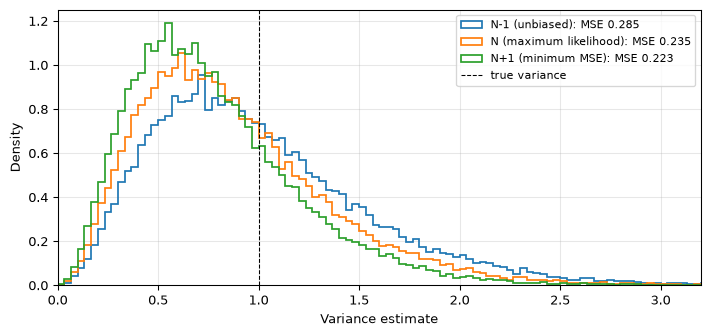
The textbook case is estimating the variance of a Gaussian from $N$ samples when the mean is also unknown. Let $S = \sum_n (x[n] - \bar{x})^2$. Dividing by $N-1$ gives the familiar unbiased estimator (Bessel’s correction); dividing by $N$ gives the maximum likelihood estimate, which is biased low. Neither minimises MSE. Writing $\hat{\sigma}^2_c = cS$ and using $E[S] = (N-1)\sigma^2$ with $\operatorname{var}(S) = 2(N-1)\sigma^4$:

\[\operatorname{MSE}(c) = \underbrace{c^2\, 2(N-1)\sigma^4}_{\text{variance}} + \underbrace{\left(c(N-1) - 1\right)^2 \sigma^4}_{\text{bias}^2}\]

Setting the derivative to zero gives $c(N+1) = 1$: the MSE-optimal divisor is $N+1$, more biased than either standard choice.

rng = np.random.default_rng(11)
N, sigma2, n_trials = 8, 1.0, 40_000

x = rng.normal(0.0, np.sqrt(sigma2), size=(n_trials, N))
S = ((x - x.mean(axis=1, keepdims=True)) ** 2).sum(axis=1)

fig, ax = plt.subplots(figsize=(7.5, 3.6))
rows = []
for label, divisor, color in [("N-1 (unbiased)", N - 1, 'C0'),
                              ("N (maximum likelihood)", N, 'C1'),
                              ("N+1 (minimum MSE)", N + 1, 'C2')]:
    est = S / divisor
    bias, var, mse = bias_variance_mse(est, sigma2)
    # Closed form, for comparison with the Monte Carlo:
    c = 1.0 / divisor
    mse_theory = c**2 * 2*(N-1) * sigma2**2 + (c*(N-1) - 1)**2 * sigma2**2
    rows.append((label, bias, var, mse, mse_theory))
    ax.hist(est, bins=120, range=(0, 4), histtype='step', density=True,
            color=color, lw=1.3, label=f"{label}: MSE {mse:.3f}")
ax.axvline(sigma2, color='k', ls='--', lw=0.8, label='true variance')
ax.set_xlabel('Variance estimate'); ax.set_ylabel('Density')
ax.set_xlim(0, 3.2); ax.legend(fontsize=8); ax.grid(True, alpha=0.3)
fig.tight_layout(); plt.show()

print(f"{'estimator':>24s} {'bias':>9s} {'variance':>9s} {'MSE':>8s} {'MSE (theory)':>13s}")
for label, bias, var, mse, mse_theory in rows:
    print(f"{label:>24s} {bias:+9.4f} {var:9.4f} {mse:8.4f} {mse_theory:13.4f}")

# The caption's claims, pinned.
by_name = {r[0]: r for r in rows}
unbiased, ml, min_mse = (by_name["N-1 (unbiased)"], by_name["N (maximum likelihood)"],
                         by_name["N+1 (minimum MSE)"])
assert abs(unbiased[1]) < 0.01, "the N-1 rule should be unbiased"
assert abs(min_mse[1]) > abs(unbiased[1]), "N+1 should be the more biased rule"
assert min_mse[2] < ml[2] < unbiased[2], "variance must fall as the divisor grows"
assert min_mse[3] < ml[3] < unbiased[3], "N+1 should win on MSE, N-1 lose"
for label, bias, var, mse, mse_theory in rows:      # Monte Carlo vs closed form
    assert abs(mse - mse_theory) < 0.01, f"{label}: MSE {mse:.4f} vs theory {mse_theory:.4f}"
print(f"\nAccepting bias cuts MSE by {(1 - min_mse[3]/unbiased[3])*100:.0f}% at N = {N}.")

Figure 1: Sampling distributions of three variance estimators (N = 8 Gaussian samples, true variance 1, 40 000 trials). Dividing by N+1 shifts the distribution further from the truth than the unbiased N-1 rule, yet lands closer on average because it is so much narrower. Unbiasedness is a constraint, not a goal.

               estimator      bias  variance      MSE  MSE (theory)
          N-1 (unbiased)   -0.0025    0.2855   0.2855        0.2857
  N (maximum likelihood)   -0.1272    0.2186   0.2348        0.2344
       N+1 (minimum MSE)   -0.2242    0.1727   0.2230        0.2222

Accepting bias cuts MSE by 22% at N = 8.

The Monte Carlo matches the closed form to three decimals, and the minimum-MSE rule is about 22% better than the unbiased one at $N = 8$. The gap closes as $N$ grows, which is why the unbiased convention is harmless in practice and why it survives: with plenty of data the three estimators agree, and unbiasedness makes the algebra tractable. But with eight samples, insisting on unbiasedness costs you real accuracy.

Everything below is nevertheless framed for unbiased estimators, for a specific reason: without some constraint, “minimise the MSE” has a stupid answer. The estimator $\hat{\theta} = 7$, ignoring the data entirely, has zero variance and beats everything when $\theta$ happens to be 7. Restricting attention to unbiased estimators rules out that cheat and makes the question “how good can an estimator be?” well posed.

Consistency, and why averaging buys $\sqrt{N}$

An estimator is consistent if it converges to the truth as data accumulates: $\hat{\theta} \to \theta$ as $N \to \infty$. This is a weaker and more practical property than unbiasedness. A consistent estimator may be biased at every finite $N$, as long as the bias vanishes; an unbiased estimator may be inconsistent, which is exactly the periodogram’s problem on the PSD estimation page: it is asymptotically unbiased but its variance never shrinks, so more data never helps.

The archetype of a consistent estimator is the sample mean. For $N$ independent samples of variance $\sigma^2$,

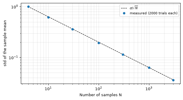
\[\operatorname{var}(\bar{x}) = \frac{\sigma^2}{N}, \qquad \text{so} \qquad \operatorname{std}(\bar{x}) = \frac{\sigma}{\sqrt{N}}\]

Its variance falls as $1/N$; its standard deviation, which is what you read off an error bar, falls only as $1/\sqrt{N}$. This is the most consequential piece of arithmetic in measurement engineering, and it is bad news dressed as good news. Halving your uncertainty costs four times the data. Improving a measurement by one decimal digit costs a hundredfold. Averaging always works and it always gets expensive, which is why so much of this workshop is about smarter alternatives: matched filters, lock-in detection, and Kalman filters all buy accuracy through structure rather than through brute repetition.

rng = np.random.default_rng(3)
sigma = 2.0
Ns = np.array([4, 10, 30, 100, 300, 1000, 3000])
measured = np.array([np.std([rng.normal(0.0, sigma, n).mean() for _ in range(2000)])
                     for n in Ns])
predicted = sigma / np.sqrt(Ns)

fig, ax = plt.subplots(figsize=(6.5, 3.6))
ax.loglog(Ns, predicted, 'k--', lw=1, label=r'$\sigma/\sqrt{N}$')
ax.loglog(Ns, measured, 'oC0', ms=5, label='measured (2000 trials each)')
ax.set_xlabel('Number of samples N'); ax.set_ylabel('std of the sample mean')
ax.grid(True, which='both', alpha=0.3); ax.legend(fontsize=8)
fig.tight_layout(); plt.show()

rel_err = np.abs(measured - predicted) / predicted
slope = np.polyfit(np.log(Ns), np.log(measured), 1)[0]
print(f"max deviation from sigma/sqrt(N): {rel_err.max()*100:.1f}%")
print(f"fitted log-log slope: {slope:.3f}  (theory -0.5)")
# The caption claims the law holds and the slope is -1/2.  With 2000 trials the
# standard error on each measured std is about 1/sqrt(2*2000) = 1.6%, so allow 8%.
assert rel_err.max() < 0.08, "measured spread should track sigma/sqrt(N)"
assert abs(slope + 0.5) < 0.03, f"log-log slope {slope:.3f} should be -1/2"

Figure 2: The square-root law. The standard deviation of the sample mean falls as σ/√N (2000 trials per point, σ = 2), a straight line of slope -1/2 on log-log axes. Reaching a tenfold improvement takes a hundredfold increase in data.

max deviation from sigma/sqrt(N): 3.1%
fitted log-log slope: -0.500  (theory -0.5)

Nature’s version of pooling noisy looks

A honeybee swarm choosing a new nest site faces an estimation problem with unreliable instruments. Individual scouts inspect candidate cavities and advertise them by dancing, and no single scout is a trustworthy judge: scouts disagree, some never visit the best site, and each assessment is noisy. The swarm’s decision nevertheless tends to land on the best available site, because the dance recruits further independent inspections in proportion to a site’s assessed quality, and the pooled evidence outruns any individual’s error (Seeley and Buhrman 1999). The analogy is loose and worth stating carefully: bees run a recruitment-and-quorum process, not an arithmetic mean, and nothing in the hive computes $1/\sqrt{N}$. What carries over is the strategy, which is the one this whole page formalises: when each look is poor, buy accuracy with many independent looks.

Prior knowledge beats more data: weighted least squares

Averaging treats every sample as equally trustworthy. Real measurements rarely are. A sensor’s noise may grow with the signal level, an integration may get noisier as a lamp warms, a range measurement gets worse with distance. If you know the noise variance $\sigma_k^2$ of each sample, you should not weight them equally.

The fit that uses this knowledge is weighted least squares. Model the measurement as a linear combination of known basis functions, $\underline{y} = \mathbf{X}\underline{\theta} + \underline{n}$, where column $j$ of the design matrix $\mathbf{X}$ holds basis function $j$ sampled at each observation point. Instead of minimising the plain sum of squared residuals, minimise the variance-normalised one:

\[\hat{\underline{\theta}} = \arg\min_{\underline{\theta}} \sum_k \frac{\left(y_k - [\mathbf{X}\underline{\theta}]_k\right)^2}{\sigma_k^2} \qquad\Longrightarrow\qquad \hat{\underline{\theta}} = \left(\mathbf{X}^T \mathbf{W} \mathbf{X}\right)^{-1} \mathbf{X}^T \mathbf{W} \underline{y}\]

with $\mathbf{W} = \operatorname{diag}(1/\sigma_k^2)$. Each residual is measured in units of its own noise, so a sample known to be noisy is allowed to miss by more without dragging the fit. The estimate’s covariance is $(\mathbf{X}^T \mathbf{W} \mathbf{X})^{-1}$, computed by weighted_least_squares alongside the fit itself.

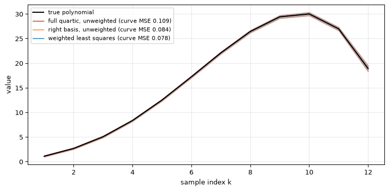
The worked example below is adapted from an exercise in the author’s archive. Twelve samples of a quartic polynomial are measured, with noise whose variance grows linearly with the sample index, $\sigma_k^2 = 0.04\,k$: across the twelve samples the variance grows twelvefold, so the last sample’s noise standard deviation ($\sqrt{0.48} \approx 0.69$) is about three and a half times the first’s ($0.2$). Two pieces of prior knowledge are available. The noise model is known, and the polynomial is known to have no constant and no quadratic term. Three fits compete:

Full quartic, unweighted: the generic polyfit-style answer, five free coefficients, all samples equal.
Right basis, unweighted: uses the structural knowledge (three coefficients) but ignores the noise model.
Weighted least squares: uses both.

k = np.arange(1, 13)
true_coeffs = np.array([1.0, 0.1, -0.008])         # coefficients of k, k^3, k^4
noise_var = 0.04 * k                                # sigma_k = 0.2*sqrt(k)

X_known = polynomial_design(k, (1, 3, 4))           # the informed basis
X_full = polynomial_design(k, (0, 1, 2, 3, 4))      # the generic quartic
f_true = X_known @ true_coeffs

rng = np.random.default_rng(2024)
n_trials = 2000
curves = {name: np.zeros((n_trials, len(k)))
          for name in ("full quartic, unweighted", "right basis, unweighted",
                       "weighted least squares")}
theta_wls = np.zeros((n_trials, 3))
theta_ols = np.zeros((n_trials, 3))
theta_full = np.zeros((n_trials, 5))

for i in range(n_trials):
    y = f_true + rng.normal(0.0, np.sqrt(noise_var))
    t_full, _ = weighted_least_squares(X_full, y, None)
    t_ols, _ = weighted_least_squares(X_known, y, None)
    t_wls, _ = weighted_least_squares(X_known, y, noise_var)
    theta_ols[i], theta_wls[i], theta_full[i] = t_ols, t_wls, t_full
    curves["full quartic, unweighted"][i] = X_full @ t_full
    curves["right basis, unweighted"][i] = X_known @ t_ols
    curves["weighted least squares"][i] = X_known @ t_wls

fig, ax = plt.subplots(figsize=(8, 4))
ax.plot(k, f_true, 'k-', lw=1.6, label='true polynomial', zorder=5)
for (name, c), color in zip(curves.items(), ['C3', 'C1', 'C0']):
    mu, sd = c.mean(axis=0), c.std(axis=0)
    ax.fill_between(k, mu - sd, mu + sd, color=color, alpha=0.22)
    ax.plot(k, mu, color=color, lw=1.1, label=f'{name} (curve MSE {np.mean((c - f_true)**2):.3f})')
ax.set_xlabel('sample index k'); ax.set_ylabel('value')
ax.legend(fontsize=8); ax.grid(True, alpha=0.3)
fig.tight_layout(); plt.show()

crlb = crlb_linear_gaussian(X_known, noise_var)
print(f"{'coefficient':>12s} {'truth':>8s} {'WLS bias':>10s} {'WLS var':>11s} "
      f"{'CRLB':>11s} {'OLS var':>11s}")
for j, (name, truth) in enumerate(zip(['k', 'k^3', 'k^4'], true_coeffs)):
    b_w, v_w, _ = bias_variance_mse(theta_wls[:, j], truth)
    _, v_o, _ = bias_variance_mse(theta_ols[:, j], truth)
    print(f"{name:>12s} {truth:8.4f} {b_w:+10.5f} {v_w:11.3e} {crlb[j, j]:11.3e} {v_o:11.3e}")

mse = {name: np.mean((c - f_true) ** 2) for name, c in curves.items()}
# Claims: WLS is unbiased, sits on the CRLB, and beats both unweighted fits.
for j, truth in enumerate(true_coeffs):
    b_w, v_w, _ = bias_variance_mse(theta_wls[:, j], truth)
    # A Monte Carlo can only resolve bias down to the standard error of the
    # mean, sqrt(var / n_trials); require the measured bias to sit inside 4
    # of those, i.e. indistinguishable from zero.
    assert abs(b_w) < 4 * np.sqrt(crlb[j, j] / n_trials), "WLS should be unbiased"
    # 2000 trials give a ~3.2% standard error on a variance, so allow 12%.
    assert abs(v_w / crlb[j, j] - 1) < 0.12, (
        f"WLS variance {v_w:.3e} should sit on the CRLB {crlb[j, j]:.3e}")
    _, v_o, _ = bias_variance_mse(theta_ols[:, j], truth)
    assert v_o > v_w, "ignoring the noise model should cost variance"
assert mse["weighted least squares"] < mse["right basis, unweighted"] \
    < mse["full quartic, unweighted"], "each piece of prior knowledge should pay"

# The prose's uncomfortable lesson: the over-parameterised fit is far worse in
# its coefficients than in its curve.  Column 1 of X_full is the k^1 term.
std_linear_full = theta_full[:, 1].std()
mse_ratio = mse["full quartic, unweighted"] / mse["weighted least squares"]
print(f"\nfull quartic, linear coefficient: std {std_linear_full:.2f} "
      f"against a true value of {true_coeffs[0]:.1f}")
print(f"yet its fitted curve is only {(mse_ratio - 1) * 100:.0f}% worse in MSE")
assert std_linear_full > true_coeffs[0], "the linear coefficient should be uninformative"
assert 1.3 < mse_ratio < 1.5, f"curve MSE ratio {mse_ratio:.2f} outside the quoted ~40%"
print("curve MSE:", {n: round(v, 4) for n, v in mse.items()})

Figure 3: Weighted least squares on twelve samples whose noise variance grows with index (2000 trials). Shaded bands are ±1 standard deviation of the fitted curve. The unweighted quartic wanders most at the low-index end, where the data is actually most trustworthy; the weighted fit using the known basis and noise model is tightest everywhere and attains the Cramér-Rao bound.

 coefficient    truth   WLS bias     WLS var        CRLB     OLS var
           k   1.0000   +0.00070   5.658e-03   5.850e-03   7.860e-03
         k^3   0.1000   -0.00000   1.291e-05   1.296e-05   1.719e-05
         k^4  -0.0080   -0.00000   7.740e-08   7.740e-08   1.001e-07

full quartic, linear coefficient: std 1.03 against a true value of 1.0
yet its fitted curve is only 40% worse in MSE
curve MSE: {'full quartic, unweighted': np.float64(0.1093), 'right basis, unweighted': np.float64(0.0836), 'weighted least squares': np.float64(0.0779)}

Two lessons, one of them uncomfortable.

The comfortable one: each piece of prior knowledge pays. Knowing which terms are absent, then knowing the noise model, each lowers the error of the fitted curve, and the weighted fit’s coefficient variances land on the Cramér-Rao bound derived in the next section, meaning no unbiased estimator could have done better with this data.

The uncomfortable one: the three fits differ far more in their coefficients than in their curves. The unweighted quartic’s estimate of the linear coefficient has a standard deviation above 1 against a true value of 1, essentially no information, while its fitted curve is only about 40% worse in MSE than the best fit. Over-parameterised fits hide their damage: the extra coefficients trade off against each other, cancelling in the fitted curve while individually meaning nothing. If you ever intend to interpret a fitted coefficient rather than merely plot the curve, this is the failure mode to fear, and it is invisible if you only look at the residuals.

The speed limit: Fisher information and the Cramér-Rao bound

So far we have compared estimators against each other. The remarkable result at the centre of estimation theory is that you can compare an estimator against the best possible estimator, without having to invent it first.

The idea is that data is informative about $\theta$ to the extent that its distribution changes when $\theta$ changes. If two very different values of $\theta$ produce nearly identical distributions of the data, no algorithm can tell them apart. Make that precise with the likelihood $p(\underline{x}; \theta)$, read as a function of $\theta$ for the data you actually observed. The Fisher information measures the average sharpness of its logarithm:

\[I(\theta) = E\left[\left(\frac{\partial \ln p(\underline{x};\theta)}{\partial \theta}\right)^2\right] = -E\left[\frac{\partial^2 \ln p(\underline{x};\theta)}{\partial \theta^2}\right]\]

A sharply peaked log-likelihood means the data pins $\theta$ down; a flat one means it barely constrains it. The Cramér-Rao lower bound (Kay 1993) then states that for any unbiased estimator, subject to mild regularity conditions on the density,

\[\operatorname{var}(\hat{\theta}) \ge \frac{1}{I(\theta)}\]

An estimator that meets the bound is called efficient; it is then also the minimum-variance unbiased estimator, and no cleverness will improve it.

Worked example: the mean of a Gaussian. Take $N$ independent samples $x[n] \sim \mathcal{N}(\theta, \sigma^2)$ with known $\sigma^2$. The log-likelihood and its derivatives are

\[\ln p = -\frac{N}{2}\ln(2\pi\sigma^2) - \frac{1}{2\sigma^2}\sum_{n=0}^{N-1}(x[n]-\theta)^2, \qquad \frac{\partial \ln p}{\partial \theta} = \frac{1}{\sigma^2}\sum_n (x[n]-\theta), \qquad \frac{\partial^2 \ln p}{\partial \theta^2} = -\frac{N}{\sigma^2}\]

The second derivative is constant, so the expectation is immediate: $I(\theta) = N/\sigma^2$ and the bound is $\sigma^2/N$. That is exactly the variance of the sample mean, so the sample mean is efficient: the $\sqrt{N}$ law is not a property of averaging, it is the physical limit of what any unbiased algorithm could extract from independent Gaussian samples. There is no signal processing trick that beats it, and knowing that is worth as much as any algorithm, because it tells you when to stop.

Note also what the bound depends on: $\sigma^2$ and $N$, and nothing else. It is computable before you take a single measurement, from the design of the experiment alone. That is how the CRLB is used in practice, sizing an integration time or an array before it is built rather than grading an estimator afterwards.

For the linear model of the previous section the same calculation gives a matrix bound, $I(\underline{\theta}) = \mathbf{X}^T\mathbf{W}\mathbf{X}$ and hence

\[\operatorname{cov}(\hat{\underline{\theta}}) \ge \left(\mathbf{X}^T\mathbf{W}\mathbf{X}\right)^{-1}\]

which is precisely the covariance that weighted least squares achieves. For a linear model in Gaussian noise, then, WLS is simultaneously the least-squares fit, the maximum likelihood estimate, and the minimum-variance unbiased estimator. Those three ideas coincide here and diverge everywhere else, which is worth remembering: the linear Gaussian case is unusually well behaved, and much of estimation theory is about what happens when it does not apply.

Two honest caveats. The bound applies to unbiased estimators, so a biased estimator can and does go below it, as the $N+1$ variance estimator did earlier. And the bound is not always attainable: an efficient estimator exists only when the score $\partial \ln p / \partial \theta$ factors as $I(\theta)(g(\underline{x}) - \theta)$, which fails for many practical problems, including frequency estimation. When it fails, the CRLB remains a valid floor but no estimator sits on it at finite $N$, and comparing against it can be unfair.

Maximum likelihood: the recipe that usually gets there

The CRLB says how good an estimator could be but not how to build one. Maximum likelihood is the closest thing to a universal recipe: choose the $\theta$ under which the data you actually observed would have been most probable.

\[\hat{\theta}_{\text{ML}} = \arg\max_{\theta} \; p(\underline{x};\theta)\]

In practice you maximise $\ln p$ instead, since it turns the products of independent samples into sums and its maximum is in the same place. The appeal is that it is mechanical: write the likelihood, differentiate, solve. The theoretical appeal is stronger. Under regularity conditions, the ML estimator is asymptotically unbiased, efficient, and Gaussian: as $N$ grows it becomes the best possible estimator and comes with its own error bars, $\hat{\theta}_{\text{ML}} \sim \mathcal{N}(\theta, 1/I(\theta))$.

The word doing the work is asymptotically. At finite $N$, an ML estimator may be biased (the $1/N$ variance estimator above is exactly the ML one, and it is biased low), and it may miss the bound. Sometimes, though, the good properties hold exactly at finite $N$, and both of this page’s running examples are such cases: the sample mean is the ML estimate of a Gaussian mean and is efficient at every $N$; weighted least squares is the ML estimate for the linear Gaussian model and sits on the bound at every $N$.

The payoff: the periodogram is (almost) maximum likelihood

The one recipe in this page’s toolkit explains a result you may already have taken on faith. On the PSD estimation page, the averaged periodogram is introduced as the obvious fix for a jumpy spectrum: chop the record into segments, transform each, average the squared magnitudes. Apply maximum likelihood to the same problem and you derive that recipe rather than guessing it, and the derivation also hands you the variance $S^2/K$, the fact that it equals the CRLB, and the $\chi^2_{2K}$ distribution behind the confidence intervals.

See Why the periodogram? It is (almost) maximum likelihood. It is worth reading that section after this page rather than before: it is this machinery applied end to end to a real estimator, including the honest caveats about which assumptions are doing the work.

Where this shows up in the rest of the workshop

The vocabulary on this page is already at work throughout the site, mostly unnamed:

PSD estimation is the fullest worked case: bias, variance, consistency, ML, and the CRLB all appear for one estimator family.
Matched filtering is the detection counterpart. It maximises output SNR for a known pulse, which is what optimality means once the question becomes “is it there?” rather than “how big is it?”.
Model-based filtering puts estimation in motion: the Kalman filter is recursive minimum-MSE estimation, and its covariance update is a running CRLB-like accounting of how much it currently knows.
Pitch detection and the Goertzel algorithm are estimators of a frequency and a bin amplitude, presented as algorithms; the frequency CRLB says how well any of them could do.
Outlier detection turns the same statistics toward decisions, and its ROC curve is where the detection half of this arc begins.

The habit worth taking away is small and portable. When you meet an estimator, ask what its distribution looks like, not just what number it returned today.

Going further

Estimating a sinusoid. Amplitude, phase, and frequency of a tone in noise is the estimation problem this workshop meets most often, and it is the next page of this arc. Amplitude and phase are linear-Gaussian and behave exactly like the examples above. Frequency is not: its bound falls as

\[\operatorname{var}(\hat{f_0}) \ge \frac{12}{(2\pi)^2\, \eta\, N(N^2-1)} \;\propto\; \frac{1}{N^3}\]

rather than $1/N$, because a longer record improves the leverage of the phase measurement as well as its averaging. Doubling the record buys a factor of 2.8 in accuracy rather than 1.4. That page also covers where the machinery here stops applying: below a threshold SNR no estimator attains the bound, because the error stops being a small perturbation and becomes an outright wrong answer.

When the noise model is wrong. Everything here assumed known, Gaussian, independent noise. Real noise is correlated (see noise whitening), sometimes heavy-tailed (see random processes), and its variance is usually estimated from the same data. Weighted least squares with estimated weights is no longer unbiased, and the CRLB computed from an assumed model is a bound on a problem you are not actually solving. How badly this bites is a question of robustness rather than of optimality, and it is the reason the outlier detection page prefers the median to the mean.

Estimators that know something in advance. If you have a prior distribution over $\theta$ rather than merely a fixed unknown value, the Bayesian machinery (MMSE estimation, the posterior mean, the Bayesian CRLB) applies, and the Kalman filter on the model-based filtering page is the best-known example in DSP. The frequentist framing on this page is the right starting point but not the only one, and the boundary between them is more a matter of what you are willing to assume than of mathematics.

References

Kay, Steven M. 1993. Fundamentals of Statistical Signal Processing, Volume i: Estimation Theory. Upper Saddle River, NJ: Prentice Hall.

Seeley, Thomas D., and Susannah C. Buhrman. 1999. “Group Decision Making in Swarms of Honey Bees.” Behavioral Ecology and Sociobiology 45 (1): 19–31. https://doi.org/10.1007/s002650050536.

--- title: "Estimation Basics" subtitle: "What makes one estimator better than another" bibliography: ../../references.bib --- Almost every page in this workshop produces a number from a noisy signal. Pitch detection returns a frequency, PSD estimation returns a spectrum, the Kalman filter returns a state, a lock-in amplifier returns an amplitude. Each of those is an **estimator**: a rule that turns data into a number that you hope is close to something real. This page is about the rules for judging such rules. When two algorithms both return "the frequency", which one is better, and better in what sense? Is there a limit to how well *any* algorithm could do with the data you have, and how would you know when you had reached it? These questions have precise answers, and the answers are surprisingly practical: they tell you when to stop optimising code and start buying a better sensor. ::: {.callout-note title="Prerequisites"} [Noise and SNR](../../basics/03-noise-snr.qmd) (variance, Gaussian noise, averaging) and comfort with basic probability (expectation, variance, the Gaussian density). The Cramér-Rao section uses derivatives of a log-likelihood; the surrounding prose says what each one means, so you can follow the argument without doing the calculus yourself. ::: ::: {.callout-tip title="This is the opening page of an arc"} Estimation and detection is a thread through several topics: measuring a quantity despite noise, and deciding whether something is there at all. This page sets up the vocabulary and the limits; the pages that follow apply them to sinusoids, delays, and detection decisions. Where a later piece is not yet written, the pointer says so. ::: ```{python} #| echo: false import numpy as np import matplotlib.pyplot as plt from estimation import (bias_variance_mse, weighted_least_squares, crlb_linear_gaussian, polynomial_design) ``` <hr> ## An estimator is a random variable Write the thing you want to know as $\theta$: an amplitude, a delay, a frequency, a noise power. You do not observe $\theta$. You observe data $\underline{x} = (x[0], \ldots, x[N-1])$ whose statistics depend on it. An **estimator** is any function of the data, $\hat{\theta} = g(\underline{x})$, intended to approximate $\theta$. The single most useful habit in this subject is to remember that $\hat{\theta}$ is *itself a random variable*. Run the same experiment tomorrow and the noise differs, so the estimate differs. It has a distribution, and every question about estimator quality is a question about that distribution: where is it centred, how wide is it, and does it tighten as you collect more data? Three quantities answer those questions. **Bias** is the offset of the centre: $b(\hat{\theta}) = E[\hat{\theta}] - \theta$. An estimator with zero bias is right *on average*, which is not the same as being right. **Variance** is the width: $\operatorname{var}(\hat{\theta}) = E\left[(\hat{\theta} - E[\hat{\theta}])^2\right]$. It measures how much your answer would jump around if you repeated the measurement. **Mean squared error** combines them, measuring distance from the truth rather than from the average estimate: $$\operatorname{MSE}(\hat{\theta}) = E\left[(\hat{\theta} - \theta)^2\right] = b(\hat{\theta})^2 + \operatorname{var}(\hat{\theta})$$ That decomposition is exact, and it is the reason "unbiased" is not a synonym for "good". MSE is a budget with two line items, and an estimator is free to spend a little bias to buy a large reduction in variance. <hr> ## Unbiased is not the same as best The textbook case is estimating the variance of a Gaussian from $N$ samples when the mean is also unknown. Let $S = \sum_n (x[n] - \bar{x})^2$. Dividing by $N-1$ gives the familiar unbiased estimator (Bessel's correction); dividing by $N$ gives the maximum likelihood estimate, which is biased low. Neither minimises MSE. Writing $\hat{\sigma}^2_c = cS$ and using $E[S] = (N-1)\sigma^2$ with $\operatorname{var}(S) = 2(N-1)\sigma^4$: $$\operatorname{MSE}(c) = \underbrace{c^2\, 2(N-1)\sigma^4}_{\text{variance}} + \underbrace{\left(c(N-1) - 1\right)^2 \sigma^4}_{\text{bias}^2}$$ Setting the derivative to zero gives $c(N+1) = 1$: the MSE-optimal divisor is $N+1$, more biased than either standard choice. ```{python} #| label: fig-bias-variance #| fig-cap: "Sampling distributions of three variance estimators (N = 8 Gaussian samples, true variance 1, 40 000 trials). Dividing by N+1 shifts the distribution further from the truth than the unbiased N-1 rule, yet lands closer on average because it is so much narrower. Unbiasedness is a constraint, not a goal." rng = np.random.default_rng(11) N, sigma2, n_trials = 8, 1.0, 40_000 x = rng.normal(0.0, np.sqrt(sigma2), size=(n_trials, N)) S = ((x - x.mean(axis=1, keepdims=True)) ** 2).sum(axis=1) fig, ax = plt.subplots(figsize=(7.5, 3.6)) rows = [] for label, divisor, color in [("N-1 (unbiased)", N - 1, 'C0'), ("N (maximum likelihood)", N, 'C1'), ("N+1 (minimum MSE)", N + 1, 'C2')]: est = S / divisor bias, var, mse = bias_variance_mse(est, sigma2) # Closed form, for comparison with the Monte Carlo: c = 1.0 / divisor mse_theory = c**2 * 2*(N-1) * sigma2**2 + (c*(N-1) - 1)**2 * sigma2**2 rows.append((label, bias, var, mse, mse_theory)) ax.hist(est, bins=120, range=(0, 4), histtype='step', density=True, color=color, lw=1.3, label=f"{label}: MSE {mse:.3f}") ax.axvline(sigma2, color='k', ls='--', lw=0.8, label='true variance') ax.set_xlabel('Variance estimate'); ax.set_ylabel('Density') ax.set_xlim(0, 3.2); ax.legend(fontsize=8); ax.grid(True, alpha=0.3) fig.tight_layout(); plt.show() print(f"{'estimator':>24s} {'bias':>9s} {'variance':>9s} {'MSE':>8s} {'MSE (theory)':>13s}") for label, bias, var, mse, mse_theory in rows: print(f"{label:>24s} {bias:+9.4f} {var:9.4f} {mse:8.4f} {mse_theory:13.4f}") # The caption's claims, pinned. by_name = {r[0]: r for r in rows} unbiased, ml, min_mse = (by_name["N-1 (unbiased)"], by_name["N (maximum likelihood)"], by_name["N+1 (minimum MSE)"]) assert abs(unbiased[1]) < 0.01, "the N-1 rule should be unbiased" assert abs(min_mse[1]) > abs(unbiased[1]), "N+1 should be the more biased rule" assert min_mse[2] < ml[2] < unbiased[2], "variance must fall as the divisor grows" assert min_mse[3] < ml[3] < unbiased[3], "N+1 should win on MSE, N-1 lose" for label, bias, var, mse, mse_theory in rows: # Monte Carlo vs closed form assert abs(mse - mse_theory) < 0.01, f"{label}: MSE {mse:.4f} vs theory {mse_theory:.4f}" print(f"\nAccepting bias cuts MSE by {(1 - min_mse[3]/unbiased[3])*100:.0f}% at N = {N}.") ``` The Monte Carlo matches the closed form to three decimals, and the minimum-MSE rule is about 22% better than the unbiased one at $N = 8$. The gap closes as $N$ grows, which is why the unbiased convention is harmless in practice and why it survives: with plenty of data the three estimators agree, and unbiasedness makes the algebra tractable. But with eight samples, insisting on unbiasedness costs you real accuracy. Everything below is nevertheless framed for unbiased estimators, for a specific reason: without some constraint, "minimise the MSE" has a stupid answer. The estimator $\hat{\theta} = 7$, ignoring the data entirely, has zero variance and beats everything when $\theta$ happens to be 7. Restricting attention to unbiased estimators rules out that cheat and makes the question "how good can an estimator be?" well posed. <hr> ## Consistency, and why averaging buys $\sqrt{N}$ An estimator is **consistent** if it converges to the truth as data accumulates: $\hat{\theta} \to \theta$ as $N \to \infty$. This is a weaker and more practical property than unbiasedness. A consistent estimator may be biased at every finite $N$, as long as the bias vanishes; an unbiased estimator may be inconsistent, which is exactly the periodogram's problem on the [PSD estimation](../psd-estimation/index.qmd) page: it is asymptotically unbiased but its variance never shrinks, so more data never helps. The archetype of a consistent estimator is the sample mean. For $N$ independent samples of variance $\sigma^2$, $$\operatorname{var}(\bar{x}) = \frac{\sigma^2}{N}, \qquad \text{so} \qquad \operatorname{std}(\bar{x}) = \frac{\sigma}{\sqrt{N}}$$ Its *variance* falls as $1/N$; its *standard deviation*, which is what you read off an error bar, falls only as $1/\sqrt{N}$. This is the most consequential piece of arithmetic in measurement engineering, and it is bad news dressed as good news. Halving your uncertainty costs four times the data. Improving a measurement by one decimal digit costs a hundredfold. Averaging always works and it always gets expensive, which is why so much of this workshop is about smarter alternatives: matched filters, lock-in detection, and Kalman filters all buy accuracy through *structure* rather than through brute repetition. ```{python} #| label: fig-sqrt-n #| fig-cap: "The square-root law. The standard deviation of the sample mean falls as σ/√N (2000 trials per point, σ = 2), a straight line of slope -1/2 on log-log axes. Reaching a tenfold improvement takes a hundredfold increase in data." rng = np.random.default_rng(3) sigma = 2.0 Ns = np.array([4, 10, 30, 100, 300, 1000, 3000]) measured = np.array([np.std([rng.normal(0.0, sigma, n).mean() for _ in range(2000)]) for n in Ns]) predicted = sigma / np.sqrt(Ns) fig, ax = plt.subplots(figsize=(6.5, 3.6)) ax.loglog(Ns, predicted, 'k--', lw=1, label=r'$\sigma/\sqrt{N}$') ax.loglog(Ns, measured, 'oC0', ms=5, label='measured (2000 trials each)') ax.set_xlabel('Number of samples N'); ax.set_ylabel('std of the sample mean') ax.grid(True, which='both', alpha=0.3); ax.legend(fontsize=8) fig.tight_layout(); plt.show() rel_err = np.abs(measured - predicted) / predicted slope = np.polyfit(np.log(Ns), np.log(measured), 1)[0] print(f"max deviation from sigma/sqrt(N): {rel_err.max()*100:.1f}%") print(f"fitted log-log slope: {slope:.3f} (theory -0.5)") # The caption claims the law holds and the slope is -1/2. With 2000 trials the # standard error on each measured std is about 1/sqrt(2*2000) = 1.6%, so allow 8%. assert rel_err.max() < 0.08, "measured spread should track sigma/sqrt(N)" assert abs(slope + 0.5) < 0.03, f"log-log slope {slope:.3f} should be -1/2" ``` ::: {.callout-tip title="Nature's version of pooling noisy looks" appearance="simple"} A honeybee swarm choosing a new nest site faces an estimation problem with unreliable instruments. Individual scouts inspect candidate cavities and advertise them by dancing, and no single scout is a trustworthy judge: scouts disagree, some never visit the best site, and each assessment is noisy. The swarm's decision nevertheless tends to land on the best available site, because the dance recruits further independent inspections in proportion to a site's assessed quality, and the pooled evidence outruns any individual's error [@seeley1999group]. The analogy is loose and worth stating carefully: bees run a recruitment-and-quorum process, not an arithmetic mean, and nothing in the hive computes $1/\sqrt{N}$. What carries over is the strategy, which is the one this whole page formalises: when each look is poor, buy accuracy with many independent looks. ::: <hr> ## Prior knowledge beats more data: weighted least squares Averaging treats every sample as equally trustworthy. Real measurements rarely are. A sensor's noise may grow with the signal level, an integration may get noisier as a lamp warms, a range measurement gets worse with distance. If you *know* the noise variance $\sigma_k^2$ of each sample, you should not weight them equally. The fit that uses this knowledge is **weighted least squares**. Model the measurement as a linear combination of known basis functions, $\underline{y} = \mathbf{X}\underline{\theta} + \underline{n}$, where column $j$ of the design matrix $\mathbf{X}$ holds basis function $j$ sampled at each observation point. Instead of minimising the plain sum of squared residuals, minimise the *variance-normalised* one: $$\hat{\underline{\theta}} = \arg\min_{\underline{\theta}} \sum_k \frac{\left(y_k - [\mathbf{X}\underline{\theta}]_k\right)^2}{\sigma_k^2} \qquad\Longrightarrow\qquad \hat{\underline{\theta}} = \left(\mathbf{X}^T \mathbf{W} \mathbf{X}\right)^{-1} \mathbf{X}^T \mathbf{W} \underline{y}$$ with $\mathbf{W} = \operatorname{diag}(1/\sigma_k^2)$. Each residual is measured in units of its own noise, so a sample known to be noisy is allowed to miss by more without dragging the fit. The estimate's covariance is $(\mathbf{X}^T \mathbf{W} \mathbf{X})^{-1}$, computed by [`weighted_least_squares`](estimation.py) alongside the fit itself. The worked example below is adapted from an exercise in the author's archive. Twelve samples of a quartic polynomial are measured, with noise whose *variance grows linearly with the sample index*, $\sigma_k^2 = 0.04\,k$: across the twelve samples the variance grows twelvefold, so the last sample's noise standard deviation ($\sqrt{0.48} \approx 0.69$) is about three and a half times the first's ($0.2$). Two pieces of prior knowledge are available. The noise model is known, and the polynomial is known to have no constant and no quadratic term. Three fits compete: 1. **Full quartic, unweighted**: the generic `polyfit`-style answer, five free coefficients, all samples equal. 2. **Right basis, unweighted**: uses the structural knowledge (three coefficients) but ignores the noise model. 3. **Weighted least squares**: uses both. ```{python} #| label: fig-wls #| fig-cap: "Weighted least squares on twelve samples whose noise variance grows with index (2000 trials). Shaded bands are ±1 standard deviation of the fitted curve. The unweighted quartic wanders most at the low-index end, where the data is actually most trustworthy; the weighted fit using the known basis and noise model is tightest everywhere and attains the Cramér-Rao bound." k = np.arange(1, 13) true_coeffs = np.array([1.0, 0.1, -0.008]) # coefficients of k, k^3, k^4 noise_var = 0.04 * k # sigma_k = 0.2*sqrt(k) X_known = polynomial_design(k, (1, 3, 4)) # the informed basis X_full = polynomial_design(k, (0, 1, 2, 3, 4)) # the generic quartic f_true = X_known @ true_coeffs rng = np.random.default_rng(2024) n_trials = 2000 curves = {name: np.zeros((n_trials, len(k))) for name in ("full quartic, unweighted", "right basis, unweighted", "weighted least squares")} theta_wls = np.zeros((n_trials, 3)) theta_ols = np.zeros((n_trials, 3)) theta_full = np.zeros((n_trials, 5)) for i in range(n_trials): y = f_true + rng.normal(0.0, np.sqrt(noise_var)) t_full, _ = weighted_least_squares(X_full, y, None) t_ols, _ = weighted_least_squares(X_known, y, None) t_wls, _ = weighted_least_squares(X_known, y, noise_var) theta_ols[i], theta_wls[i], theta_full[i] = t_ols, t_wls, t_full curves["full quartic, unweighted"][i] = X_full @ t_full curves["right basis, unweighted"][i] = X_known @ t_ols curves["weighted least squares"][i] = X_known @ t_wls fig, ax = plt.subplots(figsize=(8, 4)) ax.plot(k, f_true, 'k-', lw=1.6, label='true polynomial', zorder=5) for (name, c), color in zip(curves.items(), ['C3', 'C1', 'C0']): mu, sd = c.mean(axis=0), c.std(axis=0) ax.fill_between(k, mu - sd, mu + sd, color=color, alpha=0.22) ax.plot(k, mu, color=color, lw=1.1, label=f'{name} (curve MSE {np.mean((c - f_true)**2):.3f})') ax.set_xlabel('sample index k'); ax.set_ylabel('value') ax.legend(fontsize=8); ax.grid(True, alpha=0.3) fig.tight_layout(); plt.show() crlb = crlb_linear_gaussian(X_known, noise_var) print(f"{'coefficient':>12s} {'truth':>8s} {'WLS bias':>10s} {'WLS var':>11s} " f"{'CRLB':>11s} {'OLS var':>11s}") for j, (name, truth) in enumerate(zip(['k', 'k^3', 'k^4'], true_coeffs)): b_w, v_w, _ = bias_variance_mse(theta_wls[:, j], truth) _, v_o, _ = bias_variance_mse(theta_ols[:, j], truth) print(f"{name:>12s} {truth:8.4f} {b_w:+10.5f} {v_w:11.3e} {crlb[j, j]:11.3e} {v_o:11.3e}") mse = {name: np.mean((c - f_true) ** 2) for name, c in curves.items()} # Claims: WLS is unbiased, sits on the CRLB, and beats both unweighted fits. for j, truth in enumerate(true_coeffs): b_w, v_w, _ = bias_variance_mse(theta_wls[:, j], truth) # A Monte Carlo can only resolve bias down to the standard error of the # mean, sqrt(var / n_trials); require the measured bias to sit inside 4 # of those, i.e. indistinguishable from zero. assert abs(b_w) < 4 * np.sqrt(crlb[j, j] / n_trials), "WLS should be unbiased" # 2000 trials give a ~3.2% standard error on a variance, so allow 12%. assert abs(v_w / crlb[j, j] - 1) < 0.12, ( f"WLS variance {v_w:.3e} should sit on the CRLB {crlb[j, j]:.3e}") _, v_o, _ = bias_variance_mse(theta_ols[:, j], truth) assert v_o > v_w, "ignoring the noise model should cost variance" assert mse["weighted least squares"] < mse["right basis, unweighted"] \ < mse["full quartic, unweighted"], "each piece of prior knowledge should pay" # The prose's uncomfortable lesson: the over-parameterised fit is far worse in # its coefficients than in its curve. Column 1 of X_full is the k^1 term. std_linear_full = theta_full[:, 1].std() mse_ratio = mse["full quartic, unweighted"] / mse["weighted least squares"] print(f"\nfull quartic, linear coefficient: std {std_linear_full:.2f} " f"against a true value of {true_coeffs[0]:.1f}") print(f"yet its fitted curve is only {(mse_ratio - 1) * 100:.0f}% worse in MSE") assert std_linear_full > true_coeffs[0], "the linear coefficient should be uninformative" assert 1.3 < mse_ratio < 1.5, f"curve MSE ratio {mse_ratio:.2f} outside the quoted ~40%" print("curve MSE:", {n: round(v, 4) for n, v in mse.items()}) ``` Two lessons, one of them uncomfortable. The comfortable one: each piece of prior knowledge pays. Knowing which terms are absent, then knowing the noise model, each lowers the error of the fitted curve, and the weighted fit's coefficient variances land on the Cramér-Rao bound derived in the next section, meaning no unbiased estimator could have done better with this data. The uncomfortable one: the three fits differ far more in their *coefficients* than in their *curves*. The unweighted quartic's estimate of the linear coefficient has a standard deviation above 1 against a true value of 1, essentially no information, while its fitted curve is only about 40% worse in MSE than the best fit. Over-parameterised fits hide their damage: the extra coefficients trade off against each other, cancelling in the fitted curve while individually meaning nothing. If you ever intend to *interpret* a fitted coefficient rather than merely plot the curve, this is the failure mode to fear, and it is invisible if you only look at the residuals. <hr> ## The speed limit: Fisher information and the Cramér-Rao bound So far we have compared estimators against each other. The remarkable result at the centre of estimation theory is that you can compare an estimator against *the best possible estimator*, without having to invent it first. The idea is that data is informative about $\theta$ to the extent that its distribution *changes* when $\theta$ changes. If two very different values of $\theta$ produce nearly identical distributions of the data, no algorithm can tell them apart. Make that precise with the likelihood $p(\underline{x}; \theta)$, read as a function of $\theta$ for the data you actually observed. The **Fisher information** measures the average sharpness of its logarithm: $$I(\theta) = E\left[\left(\frac{\partial \ln p(\underline{x};\theta)}{\partial \theta}\right)^2\right] = -E\left[\frac{\partial^2 \ln p(\underline{x};\theta)}{\partial \theta^2}\right]$$ A sharply peaked log-likelihood means the data pins $\theta$ down; a flat one means it barely constrains it. The **Cramér-Rao lower bound** [@kay1993fundamentals] then states that for *any* unbiased estimator, subject to mild regularity conditions on the density, $$\operatorname{var}(\hat{\theta}) \ge \frac{1}{I(\theta)}$$ An estimator that meets the bound is called **efficient**; it is then also the minimum-variance unbiased estimator, and no cleverness will improve it. **Worked example: the mean of a Gaussian.** Take $N$ independent samples $x[n] \sim \mathcal{N}(\theta, \sigma^2)$ with known $\sigma^2$. The log-likelihood and its derivatives are $$\ln p = -\frac{N}{2}\ln(2\pi\sigma^2) - \frac{1}{2\sigma^2}\sum_{n=0}^{N-1}(x[n]-\theta)^2, \qquad \frac{\partial \ln p}{\partial \theta} = \frac{1}{\sigma^2}\sum_n (x[n]-\theta), \qquad \frac{\partial^2 \ln p}{\partial \theta^2} = -\frac{N}{\sigma^2}$$ The second derivative is constant, so the expectation is immediate: $I(\theta) = N/\sigma^2$ and the bound is $\sigma^2/N$. That is exactly the variance of the sample mean, so the sample mean is efficient: the $\sqrt{N}$ law is not a property of averaging, it is the *physical limit* of what any unbiased algorithm could extract from independent Gaussian samples. There is no signal processing trick that beats it, and knowing that is worth as much as any algorithm, because it tells you when to stop. Note also what the bound depends on: $\sigma^2$ and $N$, and nothing else. It is computable *before you take a single measurement*, from the design of the experiment alone. That is how the CRLB is used in practice, sizing an integration time or an array before it is built rather than grading an estimator afterwards. For the linear model of the previous section the same calculation gives a matrix bound, $I(\underline{\theta}) = \mathbf{X}^T\mathbf{W}\mathbf{X}$ and hence $$\operatorname{cov}(\hat{\underline{\theta}}) \ge \left(\mathbf{X}^T\mathbf{W}\mathbf{X}\right)^{-1}$$ which is precisely the covariance that weighted least squares achieves. For a linear model in Gaussian noise, then, WLS is simultaneously the least-squares fit, the maximum likelihood estimate, and the minimum-variance unbiased estimator. Those three ideas coincide here and diverge everywhere else, which is worth remembering: the linear Gaussian case is unusually well behaved, and much of estimation theory is about what happens when it does not apply. Two honest caveats. The bound applies to *unbiased* estimators, so a biased estimator can and does go below it, as the $N+1$ variance estimator did earlier. And the bound is not always attainable: an efficient estimator exists only when the score $\partial \ln p / \partial \theta$ factors as $I(\theta)(g(\underline{x}) - \theta)$, which fails for many practical problems, including frequency estimation. When it fails, the CRLB remains a valid floor but no estimator sits on it at finite $N$, and comparing against it can be unfair. <hr> ## Maximum likelihood: the recipe that usually gets there The CRLB says how good an estimator could be but not how to build one. **Maximum likelihood** is the closest thing to a universal recipe: choose the $\theta$ under which the data you actually observed would have been most probable. $$\hat{\theta}_{\text{ML}} = \arg\max_{\theta} \; p(\underline{x};\theta)$$ In practice you maximise $\ln p$ instead, since it turns the products of independent samples into sums and its maximum is in the same place. The appeal is that it is mechanical: write the likelihood, differentiate, solve. The theoretical appeal is stronger. Under regularity conditions, the ML estimator is *asymptotically* unbiased, efficient, and Gaussian: as $N$ grows it becomes the best possible estimator and comes with its own error bars, $\hat{\theta}_{\text{ML}} \sim \mathcal{N}(\theta, 1/I(\theta))$. The word doing the work is *asymptotically*. At finite $N$, an ML estimator may be biased (the $1/N$ variance estimator above is exactly the ML one, and it is biased low), and it may miss the bound. Sometimes, though, the good properties hold exactly at finite $N$, and both of this page's running examples are such cases: the sample mean is the ML estimate of a Gaussian mean and is efficient at every $N$; weighted least squares is the ML estimate for the linear Gaussian model and sits on the bound at every $N$. ::: {.callout-tip title="The payoff: the periodogram is (almost) maximum likelihood"} The one recipe in this page's toolkit explains a result you may already have taken on faith. On the [PSD estimation](../psd-estimation/index.qmd) page, the averaged periodogram is introduced as the obvious fix for a jumpy spectrum: chop the record into segments, transform each, average the squared magnitudes. Apply maximum likelihood to the same problem and you *derive* that recipe rather than guessing it, and the derivation also hands you the variance $S^2/K$, the fact that it equals the CRLB, and the $\chi^2_{2K}$ distribution behind the confidence intervals. See [Why the periodogram? It is (almost) maximum likelihood](../psd-estimation/index.qmd#why-the-periodogram-it-is-almost-maximum-likelihood). It is worth reading that section after this page rather than before: it is this machinery applied end to end to a real estimator, including the honest caveats about which assumptions are doing the work. ::: <hr> ## Where this shows up in the rest of the workshop The vocabulary on this page is already at work throughout the site, mostly unnamed: - **[PSD estimation](../psd-estimation/index.qmd)** is the fullest worked case: bias, variance, consistency, ML, and the CRLB all appear for one estimator family. - **[Matched filtering](../matched-filtering/index.qmd)** is the detection counterpart. It maximises output SNR for a known pulse, which is what optimality means once the question becomes "is it there?" rather than "how big is it?". - **[Model-based filtering](../model-based-filtering/index.qmd)** puts estimation in motion: the Kalman filter is recursive minimum-MSE estimation, and its covariance update is a running CRLB-like accounting of how much it currently knows. - **[Pitch detection](../pitch-detection/index.qmd)** and **[the Goertzel algorithm](../goertzel/index.qmd)** are estimators of a frequency and a bin amplitude, presented as algorithms; the frequency CRLB says how well any of them could do. - **[Outlier detection](../outlier-detection/index.qmd)** turns the same statistics toward decisions, and its [ROC curve](../outlier-detection/index.qmd#which-detector-at-which-threshold-the-roc-curve) is where the detection half of this arc begins. The habit worth taking away is small and portable. When you meet an estimator, ask what its distribution looks like, not just what number it returned today. <hr> ## Going further **[Estimating a sinusoid](../estimating-a-sinusoid/index.qmd).** Amplitude, phase, and frequency of a tone in noise is the estimation problem this workshop meets most often, and it is the next page of this arc. Amplitude and phase are linear-Gaussian and behave exactly like the examples above. Frequency is not: its bound falls as $$\operatorname{var}(\hat{f_0}) \ge \frac{12}{(2\pi)^2\, \eta\, N(N^2-1)} \;\propto\; \frac{1}{N^3}$$ rather than $1/N$, because a longer record improves the *leverage* of the phase measurement as well as its averaging. Doubling the record buys a factor of 2.8 in accuracy rather than 1.4. That page also covers where the machinery here stops applying: below a threshold SNR no estimator attains the bound, because the error stops being a small perturbation and becomes an outright wrong answer. **When the noise model is wrong.** Everything here assumed known, Gaussian, independent noise. Real noise is correlated (see [noise whitening](../noise-whitening/index.qmd)), sometimes heavy-tailed (see [random processes](../random-processes/index.qmd)), and its variance is usually estimated from the same data. Weighted least squares with estimated weights is no longer unbiased, and the CRLB computed from an assumed model is a bound on a problem you are not actually solving. How badly this bites is a question of robustness rather than of optimality, and it is the reason the [outlier detection](../outlier-detection/index.qmd) page prefers the median to the mean. **Estimators that know something in advance.** If you have a prior distribution over $\theta$ rather than merely a fixed unknown value, the Bayesian machinery (MMSE estimation, the posterior mean, the Bayesian CRLB) applies, and the Kalman filter on the [model-based filtering](../model-based-filtering/index.qmd) page is the best-known example in DSP. The frequentist framing on this page is the right starting point but not the only one, and the boundary between them is more a matter of what you are willing to assume than of mathematics. ## References ::: {#refs} :::