Where is it? The correlation peak, its subsample refinement, and the bandwidth-times-energy speed limit
Every “where” question a signal can answer is a “when” question in disguise. A sonar range is an echo delay. A direction of arrival is the few hundred microseconds between two microphones hearing the same clap. A cable-fault location is the difference between two arrival times. This workshop has already measured delays twice without making them the subject: the bat’s matched filter reads range off a correlation peak, and the scorpion’s leg array turns inter-leg delays into a bearing. Both pages stopped at finding the peak. This page asks the estimation-theory questions: how precisely does that peak locate the delay, what physical quantities set the limit, and which estimator reaches it, then keeps going to the two situations where the textbook answer fails: echoes (GCC-PHAT) and dispersion (the centroid method).
a scaled copy of the waveform’s own autocorrelation, slid to the delay. Since \(R_{ss}\) peaks at zero, \(R_{sy}\) peaks at \(\tau\), and the estimator is “correlate and take the argmax”, which is exactly the matched filter, and (for white Gaussian noise) exactly the maximum-likelihood estimator of \(\tau\).
The passive problem is the microphone pair’s: nobody transmitted anything you know. Two sensors see the same unknown signal with different delays and independent noises,
and only the difference\(\Delta\tau\) is estimable. Cross-correlating the two channels against each other does the same job, with one honest caveat the bound section below makes precise: the reference channel is now noisy too, and that costs performance.
From the archive: a handwritten sonar example, 1990s
The sonar example is the author’s own first meeting with this problem: a handwritten stochastic-signal-theory course notebook (TU/e course 5H130; dated pages run 1991-1999) introduces the cross-correlator as a block diagram (variable delay, multiplier, integrator) and works two examples. Example 1, “Sonar”: \(Y(t) = \alpha X(t-t_1)\) gives \(R_{xy}(\tau) = \alpha R_{xx}(\tau - t_1)\), with a sketch of the known autocorrelation shape re-appearing at \(\tau = t_1\) with height \(\alpha\). Example 2, a TV-signal ghost, reappears in the echoes section below. Both are two-line applications of stationarity. The notebook is purely symbolic, though: every number on this page is new, and its delay \(t_1\) has become \(\tau\).
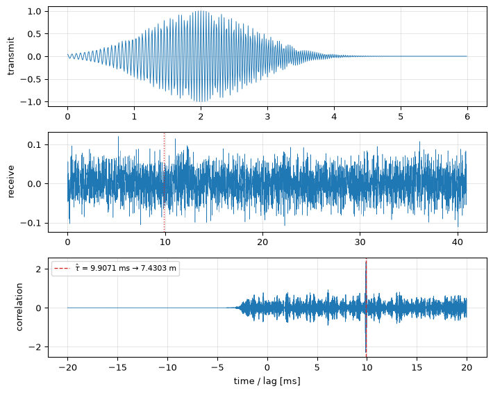
Here is the active problem with numbers on it: an ultrasonic ping in water, and an echo that a human eye cannot find in the trace.
Show the code
rng = np.random.default_rng(50)fs, c =100_000.0, 1500.0n =4096t = np.arange(n) / fstc, width =2e-3, 0.8e-3f_mid, chirp_rate =25e3, (35e3-15e3) /4e-3phase =2* np.pi * (f_mid * (t - tc) +0.5* chirp_rate * (t - tc) **2)ping = np.exp(-0.5* ((t - tc) / width) **2) * np.cos(phase)R_true =7.430# target range, metrestau_true =2* R_true / c # round-trip delay: 9.9067 msalpha =0.04# echo amplitude (28 dB loss)enr_target =100.0# echo ENR: 20 dBsigma = alpha * np.sqrt(np.sum(ping**2) / enr_target)echo = alpha * fractional_delay(ping, tau_true, fs)y = echo + sigma * rng.standard_normal(n)tau_hat = estimate_delay(ping, y, fs=fs, max_lag=2000)lags, r = cross_correlation(ping, y, max_lag=2000)fig, axes = plt.subplots(3, 1, figsize=(7.5, 6))axes[0].plot(t[:600] *1e3, ping[:600], 'C0', lw=0.7)axes[0].set_ylabel('transmit')axes[1].plot(t *1e3, y, 'C0', lw=0.4)axes[1].axvline(tau_true *1e3, color='C3', ls=':', lw=1)axes[1].set_ylabel('receive')axes[2].plot(lags / fs *1e3, r, 'C0', lw=0.6)axes[2].axvline(tau_hat *1e3, color='C3', ls='--', lw=1, label=f'$\\hat\\tau$ = {tau_hat*1e3:.4f} ms 'f'→ {c*tau_hat/2:.4f} m')axes[2].set_xlabel('time / lag [ms]'); axes[2].set_ylabel('correlation')axes[2].legend(fontsize=8)for ax in axes: ax.grid(True, alpha=0.3)fig.tight_layout(); plt.show()enr = alpha**2* np.sum(ping**2) / sigma**2print(f"echo peak / noise sigma: {alpha*np.max(np.abs(ping))/sigma:.2f} "f"(invisible), yet ENR = {10*np.log10(enr):.1f} dB")print(f"delay error: {(tau_hat - tau_true)*1e6:+.3f} us "f"= {(tau_hat - tau_true)*c/2*1e3:+.3f} mm in range")# The caption's claims, pinned: the echo is sample-wise sub-noise while# its ENR is 20 dB, and the estimate lands within 4 sigma of the CRLB# computed two sections below.assert alpha * np.max(np.abs(ping)) <1.5* sigmaassertabs(10*np.log10(enr) -20.0) <0.01sigma_crlb = np.sqrt(crlb_delay(alpha * ping, sigma**2, fs))assertabs(tau_hat - tau_true) <4* sigma_crlbassertabs(tau_hat - tau_true) <1e-6, "the caption's 'within a microsecond'"
Figure 1: Active time-delay estimation. Top: the transmitted ping, a Gaussian-windowed chirp centred on 25 kHz (sweeping roughly 17-33 kHz across its envelope). Middle: the received record; the echo, attenuated 28 dB, sits below the noise floor sample-by-sample (its peak is 1.2 noise standard deviations) and is invisible. Bottom: the cross-correlation against the known ping concentrates the echo’s total energy (ENR 20 dB) into one sharp peak at the round-trip delay of 9.907 ms, i.e. a target range of 7.430 m at c = 1500 m/s. The estimate lands within a microsecond of the truth (asserted below against the CRLB of the next sections).
echo peak / noise sigma: 1.19 (invisible), yet ENR = 20.0 dB
delay error: +0.399 us = +0.299 mm in range
The middle panel is the whole reason this field exists: per sample the echo is beneath the noise, but its total energy is a hundred times the per-sample noise variance, and correlation is the machine that trades one for the other. That trade is the pulse-compression story, and the currency it pays out in is the energy-to-noise ratio ENR \(= E_s/\sigma^2\) of the detection-theory page: the same number that decides detectability decides timing precision.
Reading the peak off the grid
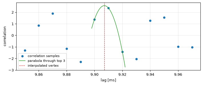
The correlation is computed at integer lags, so its argmax is quantised to the sample grid: a hard floor of \(T_s/\sqrt{12}\) rms error (2.9 µs here, over 2 mm of range) if you stop there. The fix is the same move the sinusoid page makes on the frequency axis: fit a model of the peak’s shape through the samples around the maximum and read off the vertex. The cheapest model is a parabola through three points,
Figure 2: The correlation samples around the peak of the sonar figure (dots), the parabola through the top three (line), and its vertex (dashed): the estimate moves off the integer grid. The grid alone floors the rms error at Ts/√12 = 2.9 µs; the interpolated estimator’s bound, computed next, is more than four times lower. Noise-free, the same interpolation lands within 0.05 samples of an arbitrary subsample delay (asserted), and that residual is not noise but the parabola’s model bias on a peak whose curvature is set by the 25 kHz carrier, four samples per cycle: the caveat below, already visible.
grid quantisation floor: 2.89 us rms; CRLB at this ENR: 0.63 us
noise-free interpolation error: 0.0475 samples (parabola bias, not noise)
The parabola is a model, and the interpolator-pairing lesson applies unchanged: it is only as good as its match to the true peak shape, which here is the waveform’s autocorrelation. For a smooth, oversampled peak (bandwidth comfortably below Nyquist, as in this ping) the residual bias is hundredths of a sample; for a peak only two or three samples wide the parabola’s bias grows, and the honest fixes are FFT-upsampling the correlation before interpolating, or fitting the true autocorrelation shape instead of a parabola.
How well can you possibly do? The delay CRLB
For the active problem the model is \(y[k] = s(kT_s - \tau) + w[k]\) with \(s\) known and \(w\) white Gaussian of variance \(\sigma^2\). The Fisher information for \(\tau\) follows the general Gaussian recipe: the derivative of the mean vector, squared and summed,
the second equality by Parseval, with \(f_i\) the signed DFT frequencies. Factoring out the signal energy turns this into the most quotable formula on the page:
where \(\bar\beta\) is the rms (Gabor) bandwidth in rad/s and ENR \(= E_s/\sigma^2\). Delay precision is bandwidth times the square root of energy-to-noise ratio, and nothing else: delay information lives in how fast the waveform changes, because a flat stretch of signal slid by \(d\tau\) looks identical. Sharp edges locate; slow ripples do not.
Four ways to misquote this bound
The delay CRLB is the most parameterisation-sensitive bound in this arc, and it can be silently wrong four independent ways. (1) ENR is not per-sample SNR: they differ by the window length \(N\), i.e. by \(10\log_{10} N\) dB on any axis, the same trap detection theory flags for \(P_d\) curves. (2) Noise conventions: continuous-time texts write \(1/(\bar\beta^2 \cdot 2E/N_0)\); the factor 2 is absorbed by the two-sided density \(N_0/2\) (for ideally band-limited white noise, \(\sigma^2 = (N_0/2) f_s\)), and mixing the conventions shifts the bound by 3 dB. (3) Per-sensor is not pairwise: the next section shows the two-noisy-sensor bound is the sum of the single-channel bounds: a silent factor of 2 for equal channels. (4) Signed frequencies: evaluating the Parseval sum over unsigned DFT indices \(0..N\!-\!1\) treats the upper half of the spectrum as ever-higher positive frequencies instead of negative ones, and inflates the information for any real signal: by a factor of five for the bandpass ping below, by more than fifty for a lowpass pulse (both measured; the second in test_tde.py). The remedy for all four is the same, and it is worth borrowing: check the closed form against a numerically built Fisher information rather than against your own algebra.
Show the code
# Differentiate the model numerically# (finite difference of fractionally delayed copies), build J, compare.sig2_chk =0.09j_closed =1.0/ crlb_delay(ping, sig2_chk, fs)j_numeric = delay_fisher_information_numeric(ping, sig2_chk, fs)print(f"closed-form J: {j_closed:.6e} numeric J: {j_numeric:.6e} "f"ratio {j_closed/j_numeric:.9f}")assertabs(j_closed / j_numeric -1.0) <1e-6# Trap (4), measured: the unsigned-frequency reading of the same sum.# The inflation depends on the spectrum: for this bandpass ping it is# about 5x in J (i.e. the bound 2x too tight in std); for the# lowpass pulse in test_tde.py it exceeds 50x.spec = np.abs(np.fft.fft(ping))**2w_naive =2* np.pi * np.arange(n) * fs / n # indices 0..N-1 as Hzj_naive = np.sum(w_naive**2* spec) / n / sig2_chkprint(f"unsigned-frequency reading inflates J by {j_naive/j_closed:.1f}x "f"(bound {np.sqrt(j_naive/j_closed):.1f}x too optimistic in std)")assert j_naive >3* j_closedbeta = rms_bandwidth(ping, fs)print(f"ping rms bandwidth: {beta/2/np.pi/1e3:.1f} kHz; "f"CRLB at ENR 20 dB: {sigma_crlb*1e6:.2f} us "f"= {sigma_crlb*c/2*1e3:.2f} mm of range")assertabs(1/(beta**2* enr) - sigma_crlb**2) <1e-3* sigma_crlb**2
closed-form J: 1.968556e+13   numeric J: 1.968554e+13   ratio 1.000000875
unsigned-frequency reading inflates J by 4.9x (bound 2.2x too optimistic in std)
ping rms bandwidth: 25.2 kHz; CRLB at ENR 20 dB: 0.63 us = 0.47 mm of range
Two readings of that number are worth internalising. First, accuracy is not resolution. The correlation peak of the sonar figure is about 7 cm wide at half maximum (of order \(c/2\) divided by the chirp bandwidth, the range-resolution limit for separating two targets), yet the bound for locating one target’s peak is half a millimetre: you can split a peak by far more than its width, by a factor that grows as \(\sqrt{\mathrm{ENR}}\). It is the same distinction the sinusoid page draws between the FFT bin width and the frequency CRLB.
Show the code
env = np.abs(r) / np.max(np.abs(r))width_s = np.sum(env >0.5) / fs # half-max width of |corr|print(f"correlation peak width: {width_s*1e6:.0f} us "f"({width_s*c/2*100:.1f} cm of range): resolution")print(f"CRLB on peak location: {sigma_crlb*1e6:.2f} us "f"({sigma_crlb*c/2*1e3:.2f} mm of range): accuracy")assert0.02< width_s * c /2<0.10# centimetres, not millimetresassert sigma_crlb * c /2<1e-3# sub-millimetre
correlation peak width: 90 us (6.8 cm of range): resolution
CRLB on peak location:  0.63 us (0.47 mm of range): accuracy
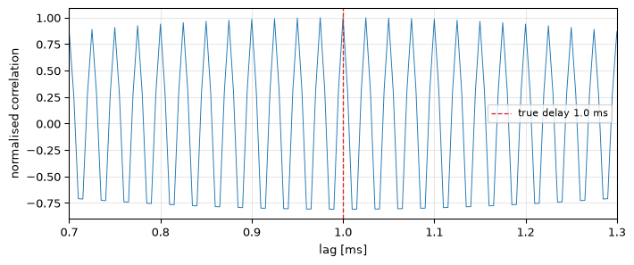
Second, \(\bar\beta\) is the second moment about zero, carrier included. A narrowband ping at a high carrier frequency has a large \(\bar\beta\) even if its envelope is slow: the delay information is riding on carrier phase. The catch is that phase only locates the delay modulo a carrier cycle:
Figure 3: Cross-correlation of a narrowband ping (2.5 kHz Gaussian envelope bandwidth on a 40 kHz carrier) with a delayed copy. The envelope is broad, but the correlation oscillates at the carrier: the true peak’s neighbours, one carrier cycle (25 µs) away, are barely lower (the tallest rival is within 0.2% of the peak, asserted). The rms bandwidth (and so the CRLB) is set almost entirely by the carrier (asserted within 3%), promising carrier-phase precision, but any noise that promotes a rival ridge produces a full-cycle error: fine accuracy, coarse ambiguity.
rms bandwidth 40.0 kHz vs carrier 40 kHz
tallest rival ridge: 0.999 of the peak, 25 us away
This accuracy-versus-ambiguity trade is why sonar and ultrasound pings are chirps rather than tone bursts (bandwidth kills the rival ridges; compare the unambiguous single peak of the first figure) and why the threshold effect, measured two sections down, bites narrowband signals at a much higher SNR.
Two noisy sensors: the bound doubles
The passive problem adds one unknown: the reference arrival time \(\tau_1\) is a nuisance parameter that must be estimated jointly with the delay difference \(\Delta\tau\). With \(A\) and \(B\) the single-channel Fisher informations of the two sensors (\(A = \bar\beta^2\,E_1/\sigma_1^2\) for the reference channel, \(B\) likewise for the delayed channel with its own received energy and noise), the \(2\times 2\) Fisher matrix for \(\theta = (\tau_1, \Delta\tau)\) works out to
\[\mathbf{J} = \begin{bmatrix} A + B & B \\ B & B \end{bmatrix}, \qquad
\operatorname{var}(\widehat{\Delta\tau}) \ge \left[\mathbf{J}^{-1}\right]_{22} = \frac{A+B}{AB} = \frac{1}{A} + \frac{1}{B}.\]
The single-channel bounds add. For equal channels the pairwise bound is exactly twice the per-sensor bound: misquoting one for the other is a silent factor of two, parameterisation trap number (3) of the callout above. The structure of \(\mathbf{J}\) explains the cost: \(\Delta\tau\) only enters through channel 2, but channel 2’s arrival time is \(\tau_1 + \Delta\tau\), so every bit of uncertainty in the reference arrival leaks straight into the difference.
From the archive: a derivation that ends “which is strange…”
The author’s own derivation behind this section, from the partial-discharge research years, sets up the DFT-domain likelihood for exactly this two-channel problem, derives the joint estimator, computes all four entries of \(\mathbf{J}\) correctly; and then, at the final step, evaluates the wrong quantity: \(1/J_{22}\) instead of \([\mathbf{J}^{-1}]_{22}\). That gives \(1/B\) alone, a bound that absurdly does not involve the reference channel’s noise at all, and the note ends mid-thought: “which is strange…”. It is: \(1/J_{22}\) is the bound you would get if \(\tau_1\) were known, and the gap between \(1/B\) and \(1/A + 1/B\) is precisely the price of estimating the reference arrival. Twenty-odd years later, the resolution is one matrix inversion long (verified numerically below and in the tests). The note carries a second subtlety, demonstrated in the previous section: its frequency sums run over DFT indices \(0..N\!-\!1\), which is only correct when read as signed frequencies. Its opening move, a minimax formulation of what happens when the noisy \(X_1\) is substituted for the unknown \(S\), remains an open question.
Show the code
# Equal channels: build the 2x2 Fisher matrix numerically (finite# differences of the actual two-channel mean vector), invert it, and# compare both candidate "bounds".s_dl = ping[:1200].copy()sig_pair =0.05h =1e-3/ fsdef two_channel_mean(tau1, dtau):return (fractional_delay(s_dl, tau1, fs), fractional_delay(s_dl, tau1 + dtau, fs))def d_mean(k): base = (2e-4, 3e-4) lo, hi =list(base), list(base) lo[k] -= h; hi[k] += h (a1, b1), (a2, b2) = two_channel_mean(*hi), two_channel_mean(*lo)return (a1 - a2) / (2*h), (b1 - b2) / (2*h)d = [d_mean(0), d_mean(1)]J = np.array([[sum(np.sum(d[i][ch] * d[j][ch]) for ch in (0, 1)) / sig_pair**2for j inrange(2)] for i inrange(2)])single = crlb_delay(s_dl, sig_pair**2, fs)pair_closed = crlb_delay_pair(s_dl, sig_pair**2, sig_pair**2, fs)bound_true = np.linalg.inv(J)[1, 1]bound_strange =1.0/ J[1, 1]print(f"[J^-1]_22 : {bound_true:.4e} s^2 "f"= {bound_true/single:.4f} x single-channel")print(f"1/J_22 ('strange') : {bound_strange:.4e} s^2 "f"= {bound_strange/single:.4f} x single-channel")assertabs(bound_true / pair_closed -1.0) <1e-4assertabs(bound_true / (2* single) -1.0) <1e-4# the factor of twoassertabs(bound_strange / single -1.0) <1e-4# tau1-known bound
[J^-1]_22          : 2.8222e-15 s^2 = 2.0000 x single-channel
1/J_22 ('strange') : 1.4111e-15 s^2 = 1.0000 x single-channel
One more honesty layer: this bound still assumes the waveform is known, with only its arrival times unknown. In the fully passive problem the signal itself is an unknown random process, and the achievable variance is worse again: the classical treatment weights each frequency by its measured coherence and is the maximum-likelihood member of the GCC family below (Knapp and Carter 1976). The known-waveform pairwise bound shipped here is the one this page can verify against a numerical Fisher matrix, and it is the honest lower envelope: no passive estimator beats it.
Measured variance against the bound, and the cliff
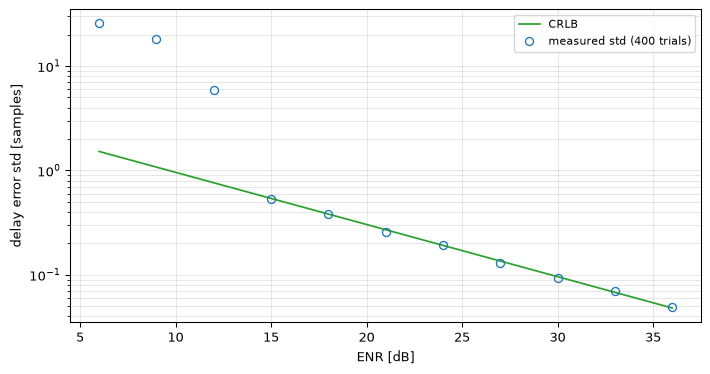
The correlation-peak estimator is the MLE, and maximum likelihood keeps its asymptotic promise: above a threshold ENR its variance sits on the CRLB. Below that threshold it falls off a cliff, and the mechanism is visible in the narrowband figure above: the true peak’s rivals (sidelobes, or just lucky noise at a distant lag) occasionally win the argmax, and one such outlier at a hundred samples’ distance does more damage than thousands of on-peak trials can average away.
Figure 4: Monte Carlo standard deviation of the correlation-peak estimator (400 trials per point, broadband test pulse, delay 7.37 samples) against the CRLB, versus ENR. Above roughly 15 dB the measured points sit on the bound (each within 25% of it, asserted): the estimator is efficient, and every extra 6 dB of ENR halves the delay error. Below the threshold the variance leaves the bound by orders of magnitude (the 6 dB point is more than 10× the bound, asserted): wrong-peak outliers, not on-peak noise, dominate. The same cliff, same cause, as the sinusoid estimator’s threshold effect.
The threshold is a design input, not a nuisance: an ultrasonic ranger that computes its link budget must check not only that the CRLB meets the spec but that the operating ENR clears the cliff: the embedded companion walks that budget for a microphone pair. And everything above assumed the peak is where the model says it is. The next two sections are about the two common ways the world breaks that assumption: echoes, and dispersion.
When the room echoes: GCC-PHAT
An echo gives the correlation function extra peaks. The author’s 1990s notebook already contains the cleanest version of this, as its second worked example, a TV signal arriving twice, direct and off a building:
side peaks at \(\pm t'\), of relative height \(\alpha/(1+\alpha^2)\) when the signal decorrelates faster than the echo delay. The notebook uses this to find the ghost delay and cancel it (\(Z(t) = Y(t) - \alpha Y(t - t')\), at the price of a weaker \(\alpha^2\) residual at \(2t'\)):
Show the code
# The notebook's TV-ghost example, executed: a colored (AR(1)) signal# plus one echo; the autocorrelation's side peak reads off the delay.rng_g = np.random.default_rng(52)x_tv = lfilter([1.0], [1.0, -0.9], rng_g.standard_normal(200_000))t_ghost, alpha_g =120, 0.4y_tv = x_tv + alpha_g * np.roll(x_tv, t_ghost)lags_g, r_g = cross_correlation(y_tv, y_tv, max_lag=300)r_g = r_g / r_g[lags_g ==0]side = r_g[lags_g == t_ghost][0]predicted = alpha_g / (1+ alpha_g**2)print(f"side peak at +{t_ghost}: {side:.4f}; "f"predicted alpha/(1+alpha^2) = {predicted:.4f}")assertabs(side - predicted) <0.02z_tv = y_tv - alpha_g * np.roll(y_tv, t_ghost)lags_z, r_z = cross_correlation(z_tv, z_tv, max_lag=300)r_z = r_z / r_z[lags_z ==0]resid = r_z[lags_z ==2* t_ghost][0]print(f"after deghosting: residual at 2t' = {resid:.4f} "f"(predicted ~ -alpha^2/(1+alpha^4) = {-alpha_g**2/(1+alpha_g**4):.4f})")assertabs(resid - (-alpha_g**2/ (1+ alpha_g**4))) <0.02
side peak at +120: 0.3494; predicted alpha/(1+alpha^2) = 0.3448
after deghosting: residual at 2t' = -0.1541 (predicted ~ -alpha^2/(1+alpha^4) = -0.1560)
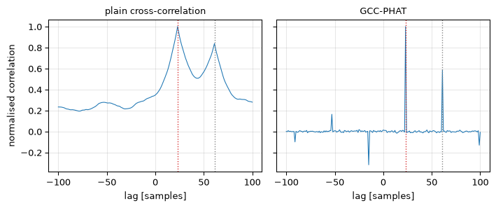
For delay estimation between two sensors, though, echoes are poison rather than signal: each multipath copy adds a correlation peak, and, worse, a colored source stretches every peak into a blob the width of the source’s own autocorrelation, until the blobs merge and the argmax lands somewhere in between. The generalised cross-correlation family (Knapp and Carter 1976) fixes this in the frequency domain: weight the cross-spectrum before inverse-transforming. The phase transform (GCC-PHAT) is the aggressive member: divide the cross-spectrum by its magnitude, keeping only phase,
Figure 5: Two-channel delay estimation with a strong echo (direct path at 23 samples, echo at 61 samples with 0.8 gain) of a heavily colored source. Left: the direct cross-correlation is a merged blob (61 lags sit above half maximum) and its interpolated peak is pulled toward the echo. Right: GCC-PHAT whitens the cross-spectrum; the two paths separate into needles at their true delays (2 lags above half maximum, thirty times sharper; at least 10× is asserted), and the interpolated direct-path estimate is an order of magnitude closer (asserted).
lags above half max: direct 61, phat 2
delay error [samples]: direct 0.013, phat 0.00115
PHAT’s price is stated by its own formula: every frequency bin gets an equal vote, including the bins that contain nothing but noise. At high SNR in a reverberant room that is exactly right (reverberation is the enemy, noise is not), which is why PHAT is the default front end for microphone-array TDOA, including the steered-beamformer localisers whose one-line mention of GCC-PHAT this section finally redeems. At low SNR the equal vote is exactly wrong, and plain correlation, which weights bins by their energy, degrades more gracefully:
Show the code
# The trade, measured: same two channels, no echo, falling SNR.rng_q = np.random.default_rng(54)src_c = lfilter([1.0], [1.0, -0.95], rng_q.standard_normal(4096))y_c = fractional_delay(src_c, d_direct)print("median |error| over 30 trials [samples]:")med = {}for snr_db in (0, -5, -10): s_n = np.sqrt(np.var(src_c) /10**(snr_db /10)) e_d, e_p = [], []for _ inrange(30): xx = src_c + s_n * rng_q.standard_normal(len(src_c)) yy = y_c + s_n * rng_q.standard_normal(len(src_c)) e_d.append(abs(estimate_delay(xx, yy, max_lag=100) - d_direct)) e_p.append(abs(estimate_delay(xx, yy, weighting='phat', max_lag=100) - d_direct)) med[snr_db] = (np.median(e_d), np.median(e_p))print(f" SNR {snr_db:+d} dB: direct {med[snr_db][0]:.2f}, "f"PHAT {med[snr_db][1]:.2f}")assert med[-10][1] > med[-10][0] # PHAT loses when noise dominates
median |error| over 30 trials [samples]:
  SNR +0 dB: direct 0.08, PHAT 0.14
  SNR -5 dB: direct 0.22, PHAT 0.30
  SNR -10 dB: direct 1.89, PHAT 2.42
Between the two extremes sits the maximum-likelihood weighting, which scales each bin by (a function of) its measured coherence, trusting frequencies where the two channels actually agree (Knapp and Carter 1976). It needs a coherence estimate, i.e. more data or stationarity; PHAT needs nothing, which is much of why it won in practice.
When there is no single delay: the centroid method
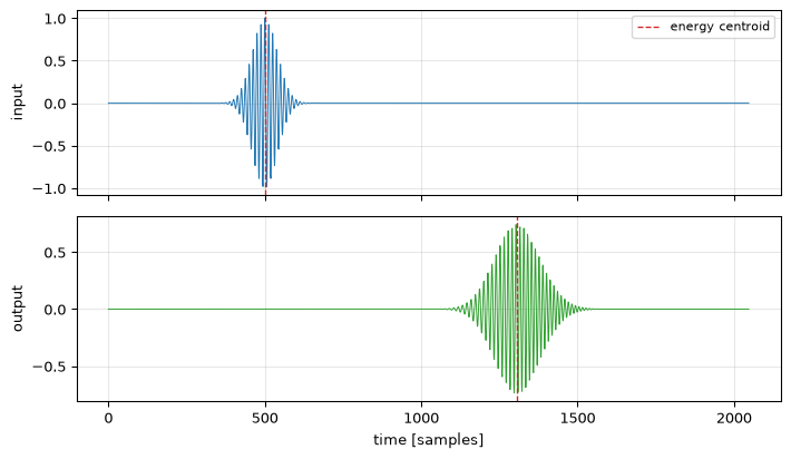
Everything so far assumed the channel delays the waveform without deforming it. A dispersive channel (a cable, a waveguide, bone, sediment) breaks that: each frequency travels at its own group velocity, the pulse smears as it propagates, and “the delay” stops being one number. Which feature of a smeared, asymmetric pulse do you time? The onset picks the fastest frequency, the peak picks a shape-dependent compromise, and the correlation peak quietly assumes the two waveforms differ only by a shift, which is now false. Every choice gives a different answer, and none of them is wrong: the question was underspecified.
This is the setting of the second first-party derivation behind this page, from the author’s partial-discharge (PD) location work: a PD pulse launched somewhere on a long cable is measured at both ends, and the difference in arrival times locates the fault, if “arrival time” can be pinned down on two pulses that have travelled different distances through a dispersive channel and no longer look alike. The proposal: time the pulse by its energy centroid(Gabor 1946),
for three reasons that the correlation peak cannot offer. It is shift-equivariant (delay the pulse by \(d\) and the centroid moves by exactly \(d\), the property that makes centroid differences measure delays). It needs no waveform model and no reference copy. And, the substantive one, it has a clean meaning under dispersion: by the moment identity \(m_1 = \frac{1}{2\pi}\int S^*(j\omega)\, j\, \frac{\partial S(j\omega)}{\partial\omega}\, d\omega\)(Cohen 1995), the centroid equals the energy-weighted mean group delay of the spectrum,
so a channel with group velocity \(v_{gr}(\omega)\) moves the centroid by the energy-weighted mean of \(x / v_{gr}(\omega)\) over the pulse’s own spectrum: a well-defined, calibratable effective delay, where “the peak” has no prediction at all.
Figure 6: A band-limited pulse before (top) and after (bottom) an all-pass dispersive channel with group delay 200 + 3·800·ω² samples: the waveform smears and grows an asymmetric tail, and peak, onset, and shape are all altered; the output is not a shifted copy of the input, so the correlation peak’s model is simply false here. The energy centroids (dashed) still measure a well-defined delay: the centroid moves by 807.14 samples, matching the channel’s |S|²-weighted mean group delay to better than 10⁻⁶ samples (asserted): the Parseval-moment identity of the archived derivation, executed.
centroid delay: 807.138494; weighted mean group delay: 807.138494
(correlation peak, whose shift model is false here: 802.78)
In the PD application the two ends’ centroid difference \(\Delta\tau_c = \tau_{c,1} - \tau_{c,2}\) becomes, after inserting the channel model, two calibration integrals weighted by the measured pulse spectra, solvable for the source position \(z\) once \(v_{gr}(\omega)\) is known from a calibration shot (George and Goodman 1988). The honest costs, so this does not read as a free lunch: the centroid is a global statistic, so noise and interference anywhere in the record bias it (window the pulse first, and the window choice re-introduces a milder version of the reference-point arbitrariness), and \(t\,|s(t)|^2\) weighting means a low-amplitude late tail moves it more than intuition expects. The correlation peak wins whenever its shift model is true; the centroid is for when dispersion has made that model a lie.
On hardware
A correlation over a handful of physically-possible lags, a three-point parabola, and an arcsine: a complete direction-of-arrival estimator fits comfortably in a microphone pair and a microcontroller, and the CRLB of this page tells you before building it how long a snippet buys how many degrees. The embedded companion builds it on both default platforms, and meets the one implementation detail that dominates everything on this page: the two channels must be sampled at the same instant, because a sequential-multiplexer skew of half a sample period is a built-in delay bias that no amount of ENR averages away.
Going further
The full GCC family. Between “no weighting” and PHAT sit Roth, SCOT, and the ML (Hannan-Thomson) weighting: all one line in gcc’s frequency loop, all trading robustness against efficiency using the estimated coherence (Knapp and Carter 1976). The ML member achieves the fully-passive CRLB asymptotically.
Threshold-region bounds. The CRLB says nothing about the cliff’s location; bounds that do (Ziv-Zakai family) predict the threshold ENR by folding in the ambiguity structure the narrowband figure displayed. The cliff measured on this page is the phenomenon they formalise.
Tracking a moving delay. A moving source makes \(\tau\) a trajectory \(\tau(t)\); feeding per-frame estimates (with their CRLB as the measurement variance) into the Kalman machinery is the classical pipeline, and recursive estimation supplies its theory. Adaptive filters estimate the delay implicitly as a moving peak in their weight vector: the adaptive-filtering page’s system-identification setting with a pure-delay plant.
Doppler. Motion also stretches the waveform. Estimating delay and Doppler jointly turns the correlation function into the two-dimensional ambiguity function, the same object behind pulse compression, now read as an estimation-theoretic trade: waveforms sharp in delay are blunt in Doppler and vice versa.
Gabor, Dennis. 1946. “Theory of Communication.”Journal of the Institution of Electrical Engineers 93 (26): 429–57.
George, J. D., and D. M. Goodman. 1988. “Estimating Time Delay and Transfer Function Parameters Using Wideband Transient Signals.” In ICASSP-88, International Conference on Acoustics, Speech, and Signal Processing, 5:2749–52. https://doi.org/10.1109/ICASSP.1988.197219.
Knapp, Charles H., and G. Clifford Carter. 1976. “The Generalized Correlation Method for Estimation of Time Delay.”IEEE Transactions on Acoustics, Speech, and Signal Processing 24 (4): 320–27. https://doi.org/10.1109/TASSP.1976.1162830.
Source Code
---title: "Time-Delay Estimation"subtitle: "Where is it? The correlation peak, its subsample refinement, and the bandwidth-times-energy speed limit"description-meta: "Finding the correlation peak and refining it below one sample, and the bandwidth-times-energy limit on how precisely an arrival can be timed."bibliography: ../../references.bib---Every "where" question a signal can answer is a "when" question in disguise. A sonar range is an echo delay. A direction of arrival is the few hundred microseconds between two microphones hearing the same clap. A cable-fault location is the difference between two arrival times. This workshop has already measured delays twice without making them the subject: the [bat's matched filter](../matched-filtering/index.qmd#application-bat-echolocation) reads range off a correlation peak, and the [scorpion's leg array](../beamforming/index.qmd#the-scorpion-simulation) turns inter-leg delays into a bearing. Both pages stopped at *finding* the peak. This page asks the estimation-theory questions: how precisely does that peak locate the delay, what physical quantities set the limit, and which estimator reaches it, then keeps going to the two situations where the textbook answer fails: echoes (GCC-PHAT) and dispersion (the centroid method).::: {.callout-note title="Prerequisites"}Part of the [estimation & detection arc](../estimation-and-detection.qmd); the overview gives the reading order.[Estimation basics](../estimation-basics/index.qmd) supplies the CRLB and maximum-likelihood machinery; [matched filtering](../matched-filtering/index.qmd) built the correlation peak this page interrogates; the [estimating-a-sinusoid page](../estimating-a-sinusoid/index.qmd#estimators-from-the-bin-grid-to-the-bound) owns the interpolate-off-the-grid move reused here on the lag axis, and its [threshold effect](../estimating-a-sinusoid/index.qmd#the-cliff-threshold-snr) returns here wearing lag-domain clothes.:::::: {.callout-tip title="Code"}The implementation is [`tde.py`](tde.py). Save [`test_tde.py`](test_tde.py) beside it and `pytest test_tde.py` runs the checks on it.:::```{python}#| echo: falseimport numpy as npimport matplotlib.pyplot as pltfrom scipy.signal import lfilterfrom tde import (cross_correlation, centroid_delay, crlb_delay, crlb_delay_pair, delay_fisher_information_numeric, estimate_delay, fractional_delay, gcc, parabolic_interpolation, rms_bandwidth, signal_centroid)```<hr>## One problem, two dresses: active and passiveThe **active** problem is sonar's: you transmitted a known waveform $s(t)$ and receive an attenuated, delayed copy in noise,$$y(t) = \alpha\, s(t - \tau) + n(t),$$and want $\tau$. Cross-correlating the received signal against the known waveform gives, in expectation,$$R_{sy}(\tau') = \alpha\, R_{ss}(\tau' - \tau):$$a scaled copy of the waveform's own autocorrelation, slid to the delay. Since $R_{ss}$ peaks at zero, $R_{sy}$ peaks at $\tau$, and the estimator is "correlate and take the argmax", which is exactly the [matched filter](../matched-filtering/index.qmd), and (for white Gaussian noise) exactly the maximum-likelihood estimator of $\tau$.The **passive** problem is the microphone pair's: nobody transmitted anything you know. Two sensors see the same unknown signal with different delays and independent noises,$$x_1(t) = s(t - \tau_1) + n_1(t), \qquad x_2(t) = \alpha\, s(t - \tau_1 - \Delta\tau) + n_2(t),$$and only the *difference* $\Delta\tau$ is estimable. Cross-correlating the two channels against each other does the same job, with one honest caveat the bound section below makes precise: the reference channel is now noisy too, and that costs performance.::: {.callout-note title="From the archive: a handwritten sonar example, 1990s"}The sonar example is the author's own first meeting with this problem: a handwritten stochastic-signal-theory course notebook (TU/e course 5H130; dated pages run 1991-1999) introduces the cross-correlator as a block diagram (variable delay, multiplier, integrator) and works two examples. Example 1, "Sonar": $Y(t) = \alpha X(t-t_1)$ gives $R_{xy}(\tau) = \alpha R_{xx}(\tau - t_1)$, with a sketch of the known autocorrelation shape re-appearing at $\tau = t_1$ with height $\alpha$. Example 2, a TV-signal ghost, reappears in the echoes section below. Both are two-line applications of stationarity. The notebook is purely symbolic, though: every number on this page is new, and its delay $t_1$ has become $\tau$.:::Here is the active problem with numbers on it: an ultrasonic ping in water, and an echo that a human eye cannot find in the trace.```{python}#| label: fig-sonar#| fig-cap: "Active time-delay estimation. Top: the transmitted ping, a Gaussian-windowed chirp centred on 25 kHz (sweeping roughly 17-33 kHz across its envelope). Middle: the received record; the echo, attenuated 28 dB, sits below the noise floor sample-by-sample (its peak is 1.2 noise standard deviations) and is invisible. Bottom: the cross-correlation against the known ping concentrates the echo's total energy (ENR 20 dB) into one sharp peak at the round-trip delay of 9.907 ms, i.e. a target range of 7.430 m at c = 1500 m/s. The estimate lands within a microsecond of the truth (asserted below against the CRLB of the next sections)."rng = np.random.default_rng(50)fs, c =100_000.0, 1500.0n =4096t = np.arange(n) / fstc, width =2e-3, 0.8e-3f_mid, chirp_rate =25e3, (35e3-15e3) /4e-3phase =2* np.pi * (f_mid * (t - tc) +0.5* chirp_rate * (t - tc) **2)ping = np.exp(-0.5* ((t - tc) / width) **2) * np.cos(phase)R_true =7.430# target range, metrestau_true =2* R_true / c # round-trip delay: 9.9067 msalpha =0.04# echo amplitude (28 dB loss)enr_target =100.0# echo ENR: 20 dBsigma = alpha * np.sqrt(np.sum(ping**2) / enr_target)echo = alpha * fractional_delay(ping, tau_true, fs)y = echo + sigma * rng.standard_normal(n)tau_hat = estimate_delay(ping, y, fs=fs, max_lag=2000)lags, r = cross_correlation(ping, y, max_lag=2000)fig, axes = plt.subplots(3, 1, figsize=(7.5, 6))axes[0].plot(t[:600] *1e3, ping[:600], 'C0', lw=0.7)axes[0].set_ylabel('transmit')axes[1].plot(t *1e3, y, 'C0', lw=0.4)axes[1].axvline(tau_true *1e3, color='C3', ls=':', lw=1)axes[1].set_ylabel('receive')axes[2].plot(lags / fs *1e3, r, 'C0', lw=0.6)axes[2].axvline(tau_hat *1e3, color='C3', ls='--', lw=1, label=f'$\\hat\\tau$ = {tau_hat*1e3:.4f} ms 'f'→ {c*tau_hat/2:.4f} m')axes[2].set_xlabel('time / lag [ms]'); axes[2].set_ylabel('correlation')axes[2].legend(fontsize=8)for ax in axes: ax.grid(True, alpha=0.3)fig.tight_layout(); plt.show()enr = alpha**2* np.sum(ping**2) / sigma**2print(f"echo peak / noise sigma: {alpha*np.max(np.abs(ping))/sigma:.2f} "f"(invisible), yet ENR = {10*np.log10(enr):.1f} dB")print(f"delay error: {(tau_hat - tau_true)*1e6:+.3f} us "f"= {(tau_hat - tau_true)*c/2*1e3:+.3f} mm in range")# The caption's claims, pinned: the echo is sample-wise sub-noise while# its ENR is 20 dB, and the estimate lands within 4 sigma of the CRLB# computed two sections below.assert alpha * np.max(np.abs(ping)) <1.5* sigmaassertabs(10*np.log10(enr) -20.0) <0.01sigma_crlb = np.sqrt(crlb_delay(alpha * ping, sigma**2, fs))assertabs(tau_hat - tau_true) <4* sigma_crlbassertabs(tau_hat - tau_true) <1e-6, "the caption's 'within a microsecond'"```The middle panel is the whole reason this field exists: *per sample* the echo is beneath the noise, but its *total energy* is a hundred times the per-sample noise variance, and correlation is the machine that trades one for the other. That trade is the [pulse-compression story](../matched-filtering/index.qmd#pulse-compression), and the currency it pays out in is the energy-to-noise ratio ENR $= E_s/\sigma^2$ of [the detection-theory page](../detection-theory/index.qmd#the-matched-filter-is-the-optimal-detector): the same number that decides detectability decides timing precision.<hr>## Reading the peak off the gridThe correlation is computed at integer lags, so its argmax is quantised to the sample grid: a hard floor of $T_s/\sqrt{12}$ rms error (2.9 µs here, over 2 mm of range) if you stop there. The fix is the same move the [sinusoid page](../estimating-a-sinusoid/index.qmd#estimators-from-the-bin-grid-to-the-bound) makes on the frequency axis: fit a model of the peak's shape through the samples around the maximum and read off the vertex. The cheapest model is a parabola through three points,$$\delta = \frac{r_{i-1} - r_{i+1}}{2\,(r_{i-1} - 2 r_i + r_{i+1})}, \qquad \hat\tau = (i + \delta)\, T_s,$$which `estimate_delay` applies by default.```{python}#| label: fig-parabola#| fig-cap: "The correlation samples around the peak of the sonar figure (dots), the parabola through the top three (line), and its vertex (dashed): the estimate moves off the integer grid. The grid alone floors the rms error at Ts/√12 = 2.9 µs; the interpolated estimator's bound, computed next, is more than four times lower. Noise-free, the same interpolation lands within 0.05 samples of an arbitrary subsample delay (asserted), and that residual is not noise but the parabola's model bias on a peak whose curvature is set by the 25 kHz carrier, four samples per cycle: the caveat below, already visible."i_pk =int(np.argmax(r))window =slice(i_pk -6, i_pk +7)delta = parabolic_interpolation(r, i_pk)par_x = np.linspace(-1.2, 1.2, 100)a_fit =0.5* (r[i_pk-1] -2*r[i_pk] + r[i_pk+1])b_fit =0.5* (r[i_pk+1] - r[i_pk-1])parab = r[i_pk] + b_fit * par_x + a_fit * par_x**2fig, ax = plt.subplots(figsize=(7.5, 3.2))ax.plot(lags[window] / fs *1e3, r[window], 'o', color='C0', ms=5, label='correlation samples')ax.plot((lags[i_pk] + par_x) / fs *1e3, parab, 'C2', lw=1.2, label='parabola through top 3')ax.axvline((lags[i_pk] + delta) / fs *1e3, color='C3', ls='--', lw=1, label='interpolated vertex')ax.set_xlabel('lag [ms]'); ax.set_ylabel('correlation')ax.legend(fontsize=8); ax.grid(True, alpha=0.3)fig.tight_layout(); plt.show()grid_floor =1/ (fs * np.sqrt(12))print(f"grid quantisation floor: {grid_floor*1e6:.2f} us rms; "f"CRLB at this ENR: {sigma_crlb*1e6:.2f} us")clean = estimate_delay(ping, alpha * fractional_delay(ping, tau_true, fs), fs=fs, max_lag=2000)print(f"noise-free interpolation error: "f"{abs(clean - tau_true)*fs:.4f} samples "f"(parabola bias, not noise)")assertabs(clean - tau_true) * fs <0.05, "the caption's exact quantity"assert grid_floor >4* sigma_crlb```The parabola is a *model*, and the [interpolator-pairing lesson](../estimating-a-sinusoid/index.qmd#estimators-from-the-bin-grid-to-the-bound) applies unchanged: it is only as good as its match to the true peak shape, which here is the waveform's autocorrelation. For a smooth, oversampled peak (bandwidth comfortably below Nyquist, as in this ping) the residual bias is hundredths of a sample; for a peak only two or three samples wide the parabola's bias grows, and the honest fixes are FFT-upsampling the correlation before interpolating, or fitting the true autocorrelation shape instead of a parabola.<hr>## How well can you possibly do? The delay CRLBFor the active problem the model is $y[k] = s(kT_s - \tau) + w[k]$ with $s$ known and $w$ white Gaussian of variance $\sigma^2$. The Fisher information for $\tau$ follows the [general Gaussian recipe](../estimation-basics/index.qmd#the-cramer-rao-lower-bound): the derivative of the mean vector, squared and summed,$$J(\tau) = \frac{1}{\sigma^2} \sum_k \left[ s'(kT_s - \tau) \right]^2 = \frac{1}{\sigma^2}\,\frac{1}{N} \sum_i (2\pi f_i)^2\, |S_i|^2,$$the second equality by Parseval, with $f_i$ the **signed** DFT frequencies. Factoring out the signal energy turns this into the most quotable formula on the page:$$\operatorname{var}(\hat\tau) \;\ge\; \frac{1}{\bar\beta^2 \cdot \mathrm{ENR}}, \qquad \bar\beta^2 = \frac{\sum_i (2\pi f_i)^2 |S_i|^2}{\sum_i |S_i|^2},$$where $\bar\beta$ is the **rms (Gabor) bandwidth** in rad/s and ENR $= E_s/\sigma^2$. Delay precision is bandwidth times the square root of energy-to-noise ratio, and nothing else: delay information lives in how fast the waveform *changes*, because a flat stretch of signal slid by $d\tau$ looks identical. Sharp edges locate; slow ripples do not.::: {.callout-warning title="Four ways to misquote this bound"}The delay CRLB is the most parameterisation-sensitive bound in this arc, and it can be silently wrong four independent ways. **(1) ENR is not per-sample SNR**: they differ by the window length $N$, i.e. by $10\log_{10} N$ dB on any axis, the same trap [detection theory](../detection-theory/index.qmd#the-matched-filter-is-the-optimal-detector) flags for $P_d$ curves. **(2) Noise conventions**: continuous-time texts write $1/(\bar\beta^2 \cdot 2E/N_0)$; the factor 2 is absorbed by the two-sided density $N_0/2$ (for ideally band-limited white noise, $\sigma^2 = (N_0/2) f_s$), and mixing the conventions shifts the bound by 3 dB. **(3) Per-sensor is not pairwise**: the next section shows the two-noisy-sensor bound is the *sum* of the single-channel bounds: a silent factor of 2 for equal channels. **(4) Signed frequencies**: evaluating the Parseval sum over unsigned DFT indices $0..N\!-\!1$ treats the upper half of the spectrum as ever-higher positive frequencies instead of negative ones, and inflates the information for any real signal: by a factor of five for the bandpass ping below, by more than fifty for a lowpass pulse (both measured; the second in [`test_tde.py`](test_tde.py)). The remedy for all four is the same, and it is worth borrowing: check the closed form against a numerically built Fisher information rather than against your own algebra.:::```{python}#| label: crlb-check# Differentiate the model numerically# (finite difference of fractionally delayed copies), build J, compare.sig2_chk =0.09j_closed =1.0/ crlb_delay(ping, sig2_chk, fs)j_numeric = delay_fisher_information_numeric(ping, sig2_chk, fs)print(f"closed-form J: {j_closed:.6e} numeric J: {j_numeric:.6e} "f"ratio {j_closed/j_numeric:.9f}")assertabs(j_closed / j_numeric -1.0) <1e-6# Trap (4), measured: the unsigned-frequency reading of the same sum.# The inflation depends on the spectrum: for this bandpass ping it is# about 5x in J (i.e. the bound 2x too tight in std); for the# lowpass pulse in test_tde.py it exceeds 50x.spec = np.abs(np.fft.fft(ping))**2w_naive =2* np.pi * np.arange(n) * fs / n # indices 0..N-1 as Hzj_naive = np.sum(w_naive**2* spec) / n / sig2_chkprint(f"unsigned-frequency reading inflates J by {j_naive/j_closed:.1f}x "f"(bound {np.sqrt(j_naive/j_closed):.1f}x too optimistic in std)")assert j_naive >3* j_closedbeta = rms_bandwidth(ping, fs)print(f"ping rms bandwidth: {beta/2/np.pi/1e3:.1f} kHz; "f"CRLB at ENR 20 dB: {sigma_crlb*1e6:.2f} us "f"= {sigma_crlb*c/2*1e3:.2f} mm of range")assertabs(1/(beta**2* enr) - sigma_crlb**2) <1e-3* sigma_crlb**2```Two readings of that number are worth internalising. First, **accuracy is not resolution**. The correlation peak of the sonar figure is about 7 cm wide at half maximum (of order $c/2$ divided by the chirp bandwidth, the [range-resolution](../matched-filtering/index.qmd#range-resolution) limit for *separating two targets*), yet the bound for *locating one target's* peak is half a millimetre: you can split a peak by far more than its width, by a factor that grows as $\sqrt{\mathrm{ENR}}$. It is the same distinction the sinusoid page draws between the FFT bin width and the frequency CRLB.```{python}#| label: resolution-vs-accuracyenv = np.abs(r) / np.max(np.abs(r))width_s = np.sum(env >0.5) / fs # half-max width of |corr|print(f"correlation peak width: {width_s*1e6:.0f} us "f"({width_s*c/2*100:.1f} cm of range): resolution")print(f"CRLB on peak location: {sigma_crlb*1e6:.2f} us "f"({sigma_crlb*c/2*1e3:.2f} mm of range): accuracy")assert0.02< width_s * c /2<0.10# centimetres, not millimetresassert sigma_crlb * c /2<1e-3# sub-millimetre```Second, $\bar\beta$ is the second moment about zero, **carrier included**. A narrowband ping at a high carrier frequency has a large $\bar\beta$ even if its envelope is slow: the delay information is riding on carrier phase. The catch is that phase only locates the delay modulo a carrier cycle:```{python}#| label: fig-narrowband#| fig-cap: "Cross-correlation of a narrowband ping (2.5 kHz Gaussian envelope bandwidth on a 40 kHz carrier) with a delayed copy. The envelope is broad, but the correlation oscillates at the carrier: the true peak's neighbours, one carrier cycle (25 µs) away, are barely lower (the tallest rival is within 0.2% of the peak, asserted). The rms bandwidth (and so the CRLB) is set almost entirely by the carrier (asserted within 3%), promising carrier-phase precision, but any noise that promotes a rival ridge produces a full-cycle error: fine accuracy, coarse ambiguity."fs_nb =200_000.0n_nb =8192t_nb = np.arange(n_nb) / fs_nbf_car, w_env =40e3, 0.4e-3# 40 kHz carrier, 0.4 ms envelopeping_nb = (np.exp(-0.5* ((t_nb -8e-3) / w_env) **2)* np.cos(2* np.pi * f_car * (t_nb -8e-3)))y_nb = fractional_delay(ping_nb, 1.0e-3, fs_nb)lags_nb, r_nb = cross_correlation(ping_nb, y_nb, max_lag=600)fig, ax = plt.subplots(figsize=(7.5, 3.2))ax.plot(lags_nb / fs_nb *1e3, r_nb / np.max(r_nb), 'C0', lw=0.7)ax.axvline(1.0, color='C3', ls='--', lw=1, label='true delay 1.0 ms')ax.set_xlim(0.7, 1.3)ax.set_xlabel('lag [ms]'); ax.set_ylabel('normalised correlation')ax.legend(fontsize=8); ax.grid(True, alpha=0.3)fig.tight_layout(); plt.show()beta_nb = rms_bandwidth(ping_nb, fs_nb)print(f"rms bandwidth {beta_nb/2/np.pi/1e3:.1f} kHz vs carrier {f_car/1e3:.0f} kHz")i0 =int(np.argmax(r_nb))rivals = np.abs(np.concatenate([r_nb[:i0-2], r_nb[i0+3:]])) / r_nb[i0]print(f"tallest rival ridge: {rivals.max():.3f} of the peak, "f"{1/f_car*1e6:.0f} us away")assertabs(beta_nb -2*np.pi*f_car) <0.03*2*np.pi*f_carassert0.998< rivals.max() <1.0```This accuracy-versus-ambiguity trade is why sonar and ultrasound pings are chirps rather than tone bursts (bandwidth kills the rival ridges; compare the unambiguous single peak of the first figure) and why the threshold effect, measured two sections down, bites narrowband signals at a much higher SNR.<hr>## Two noisy sensors: the bound doublesThe passive problem adds one unknown: the reference arrival time $\tau_1$ is a nuisance parameter that must be estimated jointly with the delay difference $\Delta\tau$. With $A$ and $B$ the single-channel Fisher informations of the two sensors ($A = \bar\beta^2\,E_1/\sigma_1^2$ for the reference channel, $B$ likewise for the delayed channel with its own received energy and noise), the $2\times 2$ Fisher matrix for $\theta = (\tau_1, \Delta\tau)$ works out to$$\mathbf{J} = \begin{bmatrix} A + B & B \\ B & B \end{bmatrix}, \qquad\operatorname{var}(\widehat{\Delta\tau}) \ge \left[\mathbf{J}^{-1}\right]_{22} = \frac{A+B}{AB} = \frac{1}{A} + \frac{1}{B}.$$The single-channel bounds **add**. For equal channels the pairwise bound is exactly twice the per-sensor bound: misquoting one for the other is a silent factor of two, parameterisation trap number (3) of the callout above. The structure of $\mathbf{J}$ explains the cost: $\Delta\tau$ only enters through channel 2, but channel 2's arrival time is $\tau_1 + \Delta\tau$, so every bit of uncertainty in the reference arrival leaks straight into the difference.::: {.callout-note title='From the archive: a derivation that ends "which is strange..."'}The author's own derivation behind this section, from the partial-discharge research years, sets up the DFT-domain likelihood for exactly this two-channel problem, derives the joint estimator, computes all four entries of $\mathbf{J}$ correctly; and then, at the final step, evaluates the wrong quantity: $1/J_{22}$ instead of $[\mathbf{J}^{-1}]_{22}$. That gives $1/B$ alone, a bound that absurdly does not involve the reference channel's noise at all, and the note ends mid-thought: *"which is strange..."*. It is: $1/J_{22}$ is the bound you would get if $\tau_1$ were **known**, and the gap between $1/B$ and $1/A + 1/B$ is precisely the price of estimating the reference arrival. Twenty-odd years later, the resolution is one matrix inversion long (verified numerically below and in the tests). The note carries a second subtlety, demonstrated in the previous section: its frequency sums run over DFT indices $0..N\!-\!1$, which is only correct when read as *signed* frequencies. Its opening move, a minimax formulation of what happens when the noisy $X_1$ is substituted for the unknown $S$, remains an open question.:::```{python}#| label: pairwise-check# Equal channels: build the 2x2 Fisher matrix numerically (finite# differences of the actual two-channel mean vector), invert it, and# compare both candidate "bounds".s_dl = ping[:1200].copy()sig_pair =0.05h =1e-3/ fsdef two_channel_mean(tau1, dtau):return (fractional_delay(s_dl, tau1, fs), fractional_delay(s_dl, tau1 + dtau, fs))def d_mean(k): base = (2e-4, 3e-4) lo, hi =list(base), list(base) lo[k] -= h; hi[k] += h (a1, b1), (a2, b2) = two_channel_mean(*hi), two_channel_mean(*lo)return (a1 - a2) / (2*h), (b1 - b2) / (2*h)d = [d_mean(0), d_mean(1)]J = np.array([[sum(np.sum(d[i][ch] * d[j][ch]) for ch in (0, 1)) / sig_pair**2for j inrange(2)] for i inrange(2)])single = crlb_delay(s_dl, sig_pair**2, fs)pair_closed = crlb_delay_pair(s_dl, sig_pair**2, sig_pair**2, fs)bound_true = np.linalg.inv(J)[1, 1]bound_strange =1.0/ J[1, 1]print(f"[J^-1]_22 : {bound_true:.4e} s^2 "f"= {bound_true/single:.4f} x single-channel")print(f"1/J_22 ('strange') : {bound_strange:.4e} s^2 "f"= {bound_strange/single:.4f} x single-channel")assertabs(bound_true / pair_closed -1.0) <1e-4assertabs(bound_true / (2* single) -1.0) <1e-4# the factor of twoassertabs(bound_strange / single -1.0) <1e-4# tau1-known bound```One more honesty layer: this bound still assumes the *waveform* is known, with only its arrival times unknown. In the fully passive problem the signal itself is an unknown random process, and the achievable variance is worse again: the classical treatment weights each frequency by its measured coherence and is the maximum-likelihood member of the GCC family below [@knapp1976generalized]. The known-waveform pairwise bound shipped here is the one this page can verify against a numerical Fisher matrix, and it is the honest lower envelope: no passive estimator beats it.<hr>## Measured variance against the bound, and the cliffThe correlation-peak estimator is the MLE, and maximum likelihood keeps its [asymptotic promise](../estimation-basics/index.qmd#maximum-likelihood-the-recipe-that-approaches-the-bound): above a threshold ENR its variance sits on the CRLB. Below that threshold it falls off a cliff, and the mechanism is visible in the narrowband figure above: the true peak's rivals (sidelobes, or just lucky noise at a distant lag) occasionally win the argmax, and one such outlier at a hundred samples' distance does more damage than thousands of on-peak trials can average away.```{python}#| label: fig-efficiency#| fig-cap: "Monte Carlo standard deviation of the correlation-peak estimator (400 trials per point, broadband test pulse, delay 7.37 samples) against the CRLB, versus ENR. Above roughly 15 dB the measured points sit on the bound (each within 25% of it, asserted): the estimator is efficient, and every extra 6 dB of ENR halves the delay error. Below the threshold the variance leaves the bound by orders of magnitude (the 6 dB point is more than 10× the bound, asserted): wrong-peak outliers, not on-peak noise, dominate. The same cliff, same cause, as the sinusoid estimator's threshold effect."def test_pulse(n=512): tt = np.arange(n, dtype=float) tc_ =0.5* n rate =0.15/ (0.8* n) ph =2* np.pi * (0.05* (tt - tc_) + rate * (tt - tc_)**2)return np.exp(-0.5* ((tt - tc_) / (0.06* n))**2) * np.cos(ph)rng_mc = np.random.default_rng(51)s_mc = test_pulse()d_true =7.37s_del = fractional_delay(s_mc, d_true)enr_db_grid = np.arange(6, 37, 3)meas, bound = [], []for edb in enr_db_grid: s2 = np.sum(s_mc**2) /10**(edb /10) est = [estimate_delay(s_mc, s_del + rng_mc.standard_normal(len(s_mc))* np.sqrt(s2), max_lag=60)for _ inrange(400)] meas.append(np.std(est)) bound.append(np.sqrt(crlb_delay(s_mc, s2)))meas, bound = np.array(meas), np.array(bound)fig, ax = plt.subplots(figsize=(7.5, 4))ax.semilogy(enr_db_grid, bound, 'C2', lw=1.3, label='CRLB')ax.semilogy(enr_db_grid, meas, 'o', color='C0', mfc='none', label='measured std (400 trials)')ax.set_xlabel('ENR [dB]'); ax.set_ylabel('delay error std [samples]')ax.legend(fontsize=8); ax.grid(True, alpha=0.3, which='both')fig.tight_layout(); plt.show()hi = enr_db_grid >=15print("std/CRLB ratio:",", ".join(f"{e} dB: {m/b:.2f}"for e, m, binzip(enr_db_grid, meas, bound)))assert np.all(np.abs(meas[hi] / bound[hi] -1.0) <0.25)assert meas[0] / bound[0] >10```The threshold is a *design input*, not a nuisance: an ultrasonic ranger that computes its link budget must check not only that the CRLB meets the spec but that the operating ENR clears the cliff: the [embedded companion](embedded.qmd) walks that budget for a microphone pair. And everything above assumed the peak is where the model says it is. The next two sections are about the two common ways the world breaks that assumption: echoes, and dispersion.<hr>## When the room echoes: GCC-PHATAn echo gives the correlation function extra peaks. The author's 1990s notebook already contains the cleanest version of this, as its second worked example, a TV signal arriving twice, direct and off a building:$$Y(t) = X(t) + \alpha X(t - t'), \qquadR_{yy}(\tau) = (1 + \alpha^2) R_{xx}(\tau) + \alpha R_{xx}(\tau + t') + \alpha R_{xx}(\tau - t'):$$side peaks at $\pm t'$, of relative height $\alpha/(1+\alpha^2)$ when the signal decorrelates faster than the echo delay. The notebook uses this to *find* the ghost delay and cancel it ($Z(t) = Y(t) - \alpha Y(t - t')$, at the price of a weaker $\alpha^2$ residual at $2t'$):```{python}#| label: ghost-check# The notebook's TV-ghost example, executed: a colored (AR(1)) signal# plus one echo; the autocorrelation's side peak reads off the delay.rng_g = np.random.default_rng(52)x_tv = lfilter([1.0], [1.0, -0.9], rng_g.standard_normal(200_000))t_ghost, alpha_g =120, 0.4y_tv = x_tv + alpha_g * np.roll(x_tv, t_ghost)lags_g, r_g = cross_correlation(y_tv, y_tv, max_lag=300)r_g = r_g / r_g[lags_g ==0]side = r_g[lags_g == t_ghost][0]predicted = alpha_g / (1+ alpha_g**2)print(f"side peak at +{t_ghost}: {side:.4f}; "f"predicted alpha/(1+alpha^2) = {predicted:.4f}")assertabs(side - predicted) <0.02z_tv = y_tv - alpha_g * np.roll(y_tv, t_ghost)lags_z, r_z = cross_correlation(z_tv, z_tv, max_lag=300)r_z = r_z / r_z[lags_z ==0]resid = r_z[lags_z ==2* t_ghost][0]print(f"after deghosting: residual at 2t' = {resid:.4f} "f"(predicted ~ -alpha^2/(1+alpha^4) = {-alpha_g**2/(1+alpha_g**4):.4f})")assertabs(resid - (-alpha_g**2/ (1+ alpha_g**4))) <0.02```For *delay estimation between two sensors*, though, echoes are poison rather than signal: each multipath copy adds a correlation peak, and, worse, a colored source stretches every peak into a blob the width of the source's own autocorrelation, until the blobs merge and the argmax lands somewhere in between. The **generalised cross-correlation** family [@knapp1976generalized] fixes this in the frequency domain: weight the cross-spectrum before inverse-transforming. The **phase transform** (GCC-PHAT) is the aggressive member: divide the cross-spectrum by its magnitude, keeping only phase,$$R^{\text{PHAT}}(\tau) = \int \frac{X_1^*(f)\, X_2(f)}{\left| X_1^*(f)\, X_2(f) \right|}\, e^{j2\pi f\tau}\, df,$$which whitens both the source coloring and the channel, so each propagation path collapses back toward an impulse at its own delay.```{python}#| label: fig-gccphat#| fig-cap: "Two-channel delay estimation with a strong echo (direct path at 23 samples, echo at 61 samples with 0.8 gain) of a heavily colored source. Left: the direct cross-correlation is a merged blob (61 lags sit above half maximum) and its interpolated peak is pulled toward the echo. Right: GCC-PHAT whitens the cross-spectrum; the two paths separate into needles at their true delays (2 lags above half maximum, thirty times sharper; at least 10× is asserted), and the interpolated direct-path estimate is an order of magnitude closer (asserted)."rng_p = np.random.default_rng(53)src = lfilter([1.0], [1.0, -0.95], rng_p.standard_normal(4096))d_direct, d_echo, g_echo =23.0, 61.0, 0.8x1 = src +0.02* rng_p.standard_normal(len(src))x2 = (fractional_delay(src, d_direct) + g_echo * fractional_delay(src, d_echo)+0.02* rng_p.standard_normal(len(src)))fig, axes = plt.subplots(1, 2, figsize=(7.5, 3.2), sharey=True)sharp, err = {}, {}for ax, wgt, title inzip(axes, ('direct', 'phat'), ('plain cross-correlation', 'GCC-PHAT')): lg, rr = gcc(x1, x2, weighting=wgt, max_lag=100) rr = rr / rr.max() sharp[wgt] =int(np.sum(rr >0.5)) err[wgt] =abs(estimate_delay(x1, x2, weighting=wgt, max_lag=100)- d_direct) ax.plot(lg, rr, 'C0', lw=0.8) ax.axvline(d_direct, color='C3', ls=':', lw=1) ax.axvline(d_echo, color='gray', ls=':', lw=1) ax.set_title(title, fontsize=10) ax.set_xlabel('lag [samples]') ax.grid(True, alpha=0.3)axes[0].set_ylabel('normalised correlation')fig.tight_layout(); plt.show()print(f"lags above half max: direct {sharp['direct']}, phat {sharp['phat']}")print(f"delay error [samples]: direct {err['direct']:.3f}, "f"phat {err['phat']:.5f}")assert sharp['phat'] *10<= sharp['direct']assert err['phat'] *10< err['direct'] and err['direct'] <0.1```PHAT's price is stated by its own formula: every frequency bin gets an equal vote, including the bins that contain nothing but noise. At high SNR in a reverberant room that is exactly right (reverberation *is* the enemy, noise is not), which is why PHAT is the default front end for microphone-array TDOA, including the [steered-beamformer localisers](../beamforming/index.qmd) whose one-line mention of GCC-PHAT this section finally redeems. At low SNR the equal vote is exactly wrong, and plain correlation, which weights bins by their energy, degrades more gracefully:```{python}#| label: phat-price# The trade, measured: same two channels, no echo, falling SNR.rng_q = np.random.default_rng(54)src_c = lfilter([1.0], [1.0, -0.95], rng_q.standard_normal(4096))y_c = fractional_delay(src_c, d_direct)print("median |error| over 30 trials [samples]:")med = {}for snr_db in (0, -5, -10): s_n = np.sqrt(np.var(src_c) /10**(snr_db /10)) e_d, e_p = [], []for _ inrange(30): xx = src_c + s_n * rng_q.standard_normal(len(src_c)) yy = y_c + s_n * rng_q.standard_normal(len(src_c)) e_d.append(abs(estimate_delay(xx, yy, max_lag=100) - d_direct)) e_p.append(abs(estimate_delay(xx, yy, weighting='phat', max_lag=100) - d_direct)) med[snr_db] = (np.median(e_d), np.median(e_p))print(f" SNR {snr_db:+d} dB: direct {med[snr_db][0]:.2f}, "f"PHAT {med[snr_db][1]:.2f}")assert med[-10][1] > med[-10][0] # PHAT loses when noise dominates```Between the two extremes sits the maximum-likelihood weighting, which scales each bin by (a function of) its measured coherence, trusting frequencies where the two channels actually agree [@knapp1976generalized]. It needs a coherence estimate, i.e. more data or stationarity; PHAT needs nothing, which is much of why it won in practice.<hr>## When there is no single delay: the centroid methodEverything so far assumed the channel delays the waveform without deforming it. A dispersive channel (a cable, a waveguide, bone, sediment) breaks that: each frequency travels at its own group velocity, the pulse smears as it propagates, and "the delay" stops being one number. Which feature of a smeared, asymmetric pulse do you time? The onset picks the *fastest* frequency, the peak picks a shape-dependent compromise, and the correlation peak quietly assumes the two waveforms differ only by a shift, which is now false. Every choice gives a different answer, and none of them is wrong: the question was underspecified.This is the setting of the second first-party derivation behind this page, from the author's partial-discharge (PD) location work: a PD pulse launched somewhere on a long cable is measured at both ends, and the *difference* in arrival times locates the fault, if "arrival time" can be pinned down on two pulses that have travelled different distances through a dispersive channel and no longer look alike. The proposal: time the pulse by its **energy centroid** [@gabor1946theory],$$\tau_c = \frac{m_1}{m_0} = \frac{\int t\, |s(t)|^2\, dt}{\int |s(t)|^2\, dt},$$for three reasons that the correlation peak cannot offer. It is **shift-equivariant** (delay the pulse by $d$ and the centroid moves by exactly $d$, the property that makes centroid differences measure delays). It needs **no waveform model** and no reference copy. And, the substantive one, it has a clean meaning *under* dispersion: by the moment identity $m_1 = \frac{1}{2\pi}\int S^*(j\omega)\, j\, \frac{\partial S(j\omega)}{\partial\omega}\, d\omega$ [@cohen1995time], the centroid equals the energy-weighted mean **group delay** of the spectrum,$$\tau_c = \frac{\int |S(j\omega)|^2\, \tau_{gr}(\omega)\, d\omega}{\int |S(j\omega)|^2\, d\omega}, \qquad \tau_{gr}(\omega) = -\frac{\partial \arg S(j\omega)}{\partial \omega},$$so a channel with group velocity $v_{gr}(\omega)$ moves the centroid by the energy-weighted mean of $x / v_{gr}(\omega)$ over the pulse's own spectrum: a well-defined, calibratable effective delay, where "the peak" has no prediction at all.```{python}#| label: fig-centroid#| fig-cap: "A band-limited pulse before (top) and after (bottom) an all-pass dispersive channel with group delay 200 + 3·800·ω² samples: the waveform smears and grows an asymmetric tail, and peak, onset, and shape are all altered; the output is not a shifted copy of the input, so the correlation peak's model is simply false here. The energy centroids (dashed) still measure a well-defined delay: the centroid moves by 807.14 samples, matching the channel's |S|²-weighted mean group delay to better than 10⁻⁶ samples (asserted): the Parseval-moment identity of the archived derivation, executed."n_c =2048t_c = np.arange(n_c, dtype=float)pulse = (np.exp(-0.5* ((t_c -500) /40.0)**2)* np.cos(2* np.pi *0.08* (t_c -500)))w_c =2* np.pi * np.fft.fftfreq(n_c)tau0, b3 =200.0, 800.0channel = np.exp(-1j* (tau0 * w_c + b3 * w_c**3)) # group delay tau0+3 b3 w^2out = np.fft.ifft(np.fft.fft(pulse) * channel).realcd = centroid_delay(pulse, out)spec_c = np.abs(np.fft.fft(pulse))**2gd_mean = np.sum(spec_c * (tau0 +3* b3 * w_c**2)) / np.sum(spec_c)fig, axes = plt.subplots(2, 1, figsize=(7.5, 4.4), sharex=True)axes[0].plot(t_c, pulse, 'C0', lw=0.7)axes[0].axvline(signal_centroid(pulse), color='C3', ls='--', lw=1, label='energy centroid')axes[0].set_ylabel('input'); axes[0].legend(fontsize=8)axes[1].plot(t_c, out, 'C2', lw=0.7)axes[1].axvline(signal_centroid(out), color='C3', ls='--', lw=1)axes[1].set_ylabel('output'); axes[1].set_xlabel('time [samples]')for ax in axes: ax.grid(True, alpha=0.3)fig.tight_layout(); plt.show()xc_peak = estimate_delay(pulse, out, max_lag=1500)print(f"centroid delay: {cd:.6f}; weighted mean group delay: {gd_mean:.6f}")print(f"(correlation peak, whose shift model is false here: {xc_peak:.2f})")assertabs(cd - gd_mean) <1e-6assertabs(cd -807.14) <0.01# the caption's numberequi = centroid_delay(pulse, fractional_delay(pulse, 13.71)) -13.71assertabs(equi) <1e-9# shift equivariance, exactly```In the PD application the two ends' centroid difference $\Delta\tau_c = \tau_{c,1} - \tau_{c,2}$ becomes, after inserting the channel model, two calibration integrals weighted by the measured pulse spectra, solvable for the source position $z$ once $v_{gr}(\omega)$ is known from a calibration shot [@george1988estimating]. The honest costs, so this does not read as a free lunch: the centroid is a *global* statistic, so noise and interference anywhere in the record bias it (window the pulse first, and the window choice re-introduces a milder version of the reference-point arbitrariness), and $t\,|s(t)|^2$ weighting means a low-amplitude late tail moves it more than intuition expects. The correlation peak wins whenever its shift model is true; the centroid is for when dispersion has made that model a lie.<hr>## On hardwareA correlation over a handful of physically-possible lags, a three-point parabola, and an arcsine: a complete direction-of-arrival estimator fits comfortably in a microphone pair and a microcontroller, and the CRLB of this page tells you *before building it* how long a snippet buys how many degrees. [The embedded companion](embedded.qmd) builds it on both default platforms, and meets the one implementation detail that dominates everything on this page: the two channels must be sampled at the *same instant*, because a sequential-multiplexer skew of half a sample period is a built-in delay bias that no amount of ENR averages away.<hr>## Going further**The full GCC family.** Between "no weighting" and PHAT sit Roth, SCOT, and the ML (Hannan-Thomson) weighting: all one line in `gcc`'s frequency loop, all trading robustness against efficiency using the estimated coherence [@knapp1976generalized]. The ML member achieves the fully-passive CRLB asymptotically.**Threshold-region bounds.** The CRLB says nothing about the cliff's location; bounds that do (Ziv-Zakai family) predict the threshold ENR by folding in the ambiguity structure the narrowband figure displayed. The cliff measured on this page is the phenomenon they formalise.**Tracking a moving delay.** A moving source makes $\tau$ a trajectory $\tau(t)$; feeding per-frame estimates (with their CRLB as the measurement variance) into the [Kalman machinery](../model-based-filtering/index.qmd) is the classical pipeline, and [recursive estimation](../recursive-estimation/index.qmd) supplies its theory. Adaptive filters estimate the delay implicitly as a moving peak in their weight vector: the [adaptive-filtering page's](../adaptive-filtering/index.qmd) system-identification setting with a pure-delay plant.**Doppler.** Motion also *stretches* the waveform. Estimating delay and Doppler jointly turns the correlation function into the two-dimensional ambiguity function, the same object behind [pulse compression](../matched-filtering/index.qmd#pulse-compression), now read as an estimation-theoretic trade: waveforms sharp in delay are blunt in Doppler and vice versa.## References::: {#refs}:::