Image Noise

Noise in two dimensions: models and denoising

Image noise is different from audio noise. The noise is spatial, not temporal; it is often signal-dependent (photon shot noise); and the human visual system is the ultimate judge of what denoising “should” look like: sharper is not always better if the noise texture is perceptually acceptable. This page covers the four major noise models in imaging and the denoising methods matched to each (Gonzalez and Woods 2018).

The companion module image_noise.py implements the noise models and denoising algorithms. Run pytest to verify.

Prerequisites

Noise and SNR and random processes (Poisson and Gaussian processes).

Four noise models

Gaussian: thermal and read noise

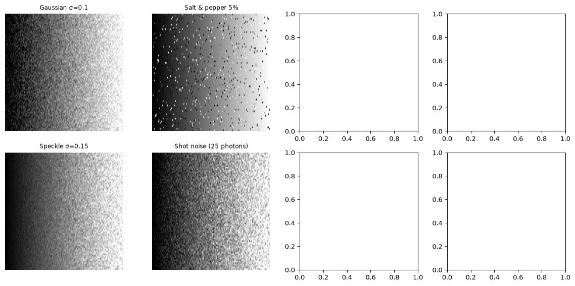
Additive, signal-independent, flat spectrum. Models CMOS sensor read noise and thermal noise in the amplifier chain. The simplest model and the baseline against which all others are compared.

Salt-and-pepper: dead pixels

Random pixels saturate to black or white. Models dead/hot pixels on a sensor and bit errors in transmission. The defining property: most pixels are uncorrupted, but the corrupted ones are at extreme values. A median filter removes it almost perfectly; a Gaussian filter smears it across neighbours.

Speckle: multiplicative noise

Signal × (1 + noise), characteristic of coherent imaging (ultrasound, synthetic aperture radar, laser). Dark regions have low absolute noise; bright regions have high absolute noise. Linear filters are poorly matched: the noise is signal-dependent.

Shot noise: photon counting

The fundamental quantum limit. Each pixel collects a random number of photons drawn from a Poisson distribution with mean equal to the expected count. Variance equals the mean: darker regions have higher relative noise ($\sqrt{\lambda}/\lambda = 1/\sqrt{\lambda}$). This is the dominant noise source in low-light imaging and the reason bigger pixels (more photons collected) give cleaner images.

img = np.tile(np.linspace(0, 1, 200), (80, 1))

fig, axes = plt.subplots(2, 4, figsize=(12, 6))
for ax_row, models in zip(axes, [
    [(add_gaussian, {'sigma': 0.1}, 'Gaussian σ=0.1'),
     (add_salt_pepper, {'prob': 0.05}, 'Salt & pepper 5%')],
    [(add_speckle, {'sigma': 0.15}, 'Speckle σ=0.15'),
     (add_shot_noise, {'peak_photons': 25}, 'Shot noise (25 photons)')]
]):
    for ax, (fn, kwargs, title) in zip(ax_row, models):
        noisy = fn(img, **kwargs, seed=42)
        ax.imshow(noisy, cmap='gray', aspect='auto', vmin=0, vmax=1)
        ax.set_title(title, fontsize=9); ax.axis('off')
fig.tight_layout(); plt.show()

Figure 1: Four noise models on a gradient test image. Top row: Gaussian, salt-and-pepper. Bottom row: speckle, shot noise (low photon count).

Denoising methods

Median filter: for salt-and-pepper

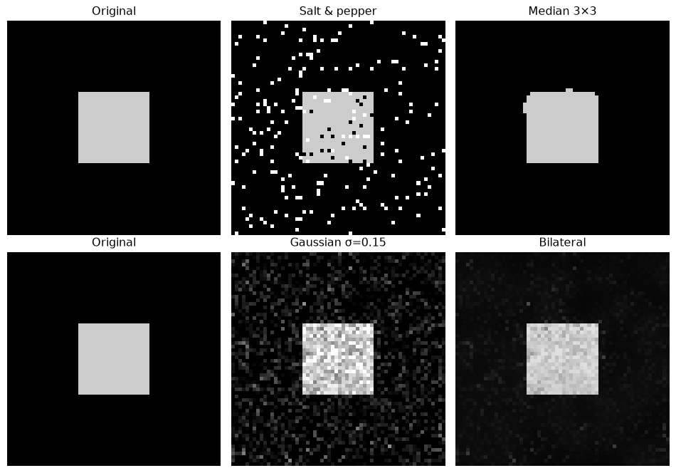
Replace each pixel with the median of its neighbourhood. Salt-and-pepper pixels are outliers and the median ignores them. A 3×3 median filter removes nearly all salt-and-pepper noise with minimal blurring: it is the textbook case of a filter matched to its noise model.

Bilateral filter: edge-preserving smoothing

Weights each neighbour by both spatial distance AND intensity difference. A pixel across an edge (similar spatial distance, very different intensity) gets near-zero weight. The result: smoothing within homogeneous regions, preservation across edges. The bilateral filter is the bridge between Gaussian smoothing (all neighbours equal) and non-local means (Buades, Coll, and Morel 2005) (all similar patches, regardless of distance).

img_checker = np.zeros((60, 60))
img_checker[20:40, 20:40] = 0.8

fig, axes = plt.subplots(2, 3, figsize=(10, 7))

# Salt-and-pepper -> median
noisy_sp = add_salt_pepper(img_checker, prob=0.1, seed=1)
axes[0, 0].imshow(img_checker, cmap='gray', vmin=0, vmax=1); axes[0, 0].set_title('Original')
axes[0, 1].imshow(noisy_sp, cmap='gray', vmin=0, vmax=1); axes[0, 1].set_title('Salt & pepper')
denoised_sp = denoise_median(noisy_sp, size=3)
axes[0, 2].imshow(denoised_sp, cmap='gray', vmin=0, vmax=1); axes[0, 2].set_title('Median 3×3')

# Gaussian -> bilateral
noisy_g = add_gaussian(img_checker, sigma=0.15, seed=1)
axes[1, 0].imshow(img_checker, cmap='gray', vmin=0, vmax=1); axes[1, 0].set_title('Original')
axes[1, 1].imshow(noisy_g, cmap='gray', vmin=0, vmax=1); axes[1, 1].set_title('Gaussian σ=0.15')
denoised_g = denoise_bilateral(noisy_g, sigma_spatial=3.0, sigma_intensity=0.2)
axes[1, 2].imshow(denoised_g, cmap='gray', vmin=0, vmax=1); axes[1, 2].set_title('Bilateral')

for ax in axes.ravel(): ax.axis('off')
fig.tight_layout(); plt.show()

Figure 2: Denoising comparison. Top: original + salt-and-pepper, median filter result. Bottom: original + Gaussian, bilateral filter result.

The honest limit

Denoising always loses something. A median filter removes salt-and-pepper noise but also erases single-pixel features. A bilateral filter preserves edges but can create cartoon-like flat regions. A wavelet denoising method (see the wavelets topic) sets a universal threshold that works well for Gaussian noise and poorly for speckle.

The right question is not “which denoiser is best” but “what information must survive the denoising step for the downstream task?” A medical image needs edges preserved; a texture classifier needs the texture statistics preserved; a face detector just needs the face.

Going further

Wavelets: VisuShrink and wavelet-domain denoising: the threshold that minimaximises MSE for Gaussian noise.
Gabor filters: spatial-frequency analysis that the visual cortex performs, relevant because good denoising respects what the human visual system notices.
Dither: the 2-D analogue of dither is Floyd-Steinberg error diffusion, spatial noise shaping for image quantisation.

References

Buades, Antoni, Bartomeu Coll, and Jean-Michel Morel. 2005. “A Non-Local Algorithm for Image Denoising.” IEEE Computer Society Conference on Computer Vision and Pattern Recognition (CVPR 2005) 2: 60–65.

Gonzalez, Rafael C., and Richard E. Woods. 2018. Digital Image Processing. 4th ed. Pearson.

--- title: "Image Noise" subtitle: "Noise in two dimensions: models and denoising" bibliography: ../../references.bib --- Image noise is different from audio noise. The noise is spatial, not temporal; it is often signal-dependent (photon shot noise); and the human visual system is the ultimate judge of what denoising "should" look like: sharper is not always better if the noise texture is perceptually acceptable. This page covers the four major noise models in imaging and the denoising methods matched to each [@gonzalez2018digital]. The companion module [`image_noise.py`](image_noise.py) implements the noise models and denoising algorithms. Run `pytest` to verify. ::: {.callout-note title="Prerequisites"} [Noise and SNR](../../basics/03-noise-snr.qmd) and [random processes](../random-processes/index.qmd) (Poisson and Gaussian processes). ::: ```{python} #| echo: false import numpy as np import matplotlib.pyplot as plt from image_noise import (add_gaussian, add_salt_pepper, add_speckle, add_shot_noise, denoise_median, denoise_bilateral) ``` <hr> ## Four noise models ### Gaussian: thermal and read noise Additive, signal-independent, flat spectrum. Models CMOS sensor read noise and thermal noise in the amplifier chain. The simplest model and the baseline against which all others are compared. ### Salt-and-pepper: dead pixels Random pixels saturate to black or white. Models dead/hot pixels on a sensor and bit errors in transmission. The defining property: most pixels are uncorrupted, but the corrupted ones are at extreme values. A median filter removes it almost perfectly; a Gaussian filter smears it across neighbours. ### Speckle: multiplicative noise Signal × (1 + noise), characteristic of coherent imaging (ultrasound, synthetic aperture radar, laser). Dark regions have low absolute noise; bright regions have high absolute noise. Linear filters are poorly matched: the noise is signal-dependent. ### Shot noise: photon counting The fundamental quantum limit. Each pixel collects a random number of photons drawn from a Poisson distribution with mean equal to the expected count. Variance equals the mean: darker regions have *higher* relative noise ($\sqrt{\lambda}/\lambda = 1/\sqrt{\lambda}$). This is the dominant noise source in low-light imaging and the reason bigger pixels (more photons collected) give cleaner images. ```{python} #| label: fig-image-noise-models #| fig-cap: "Four noise models on a gradient test image. Top row: Gaussian, salt-and-pepper. Bottom row: speckle, shot noise (low photon count)." img = np.tile(np.linspace(0, 1, 200), (80, 1)) fig, axes = plt.subplots(2, 4, figsize=(12, 6)) for ax_row, models in zip(axes, [ [(add_gaussian, {'sigma': 0.1}, 'Gaussian σ=0.1'), (add_salt_pepper, {'prob': 0.05}, 'Salt & pepper 5%')], [(add_speckle, {'sigma': 0.15}, 'Speckle σ=0.15'), (add_shot_noise, {'peak_photons': 25}, 'Shot noise (25 photons)')] ]): for ax, (fn, kwargs, title) in zip(ax_row, models): noisy = fn(img, **kwargs, seed=42) ax.imshow(noisy, cmap='gray', aspect='auto', vmin=0, vmax=1) ax.set_title(title, fontsize=9); ax.axis('off') fig.tight_layout(); plt.show() ``` <hr> ## Denoising methods ### Median filter: for salt-and-pepper Replace each pixel with the median of its neighbourhood. Salt-and-pepper pixels are outliers and the median ignores them. A 3×3 median filter removes nearly all salt-and-pepper noise with minimal blurring: it is the textbook case of a filter matched to its noise model. ### Bilateral filter: edge-preserving smoothing Weights each neighbour by both spatial distance AND intensity difference. A pixel across an edge (similar spatial distance, very different intensity) gets near-zero weight. The result: smoothing within homogeneous regions, preservation across edges. The bilateral filter is the bridge between Gaussian smoothing (all neighbours equal) and non-local means [@buades2005nonlocal] (all similar patches, regardless of distance). ```{python} #| label: fig-denoising #| fig-cap: "Denoising comparison. Top: original + salt-and-pepper, median filter result. Bottom: original + Gaussian, bilateral filter result." img_checker = np.zeros((60, 60)) img_checker[20:40, 20:40] = 0.8 fig, axes = plt.subplots(2, 3, figsize=(10, 7)) # Salt-and-pepper -> median noisy_sp = add_salt_pepper(img_checker, prob=0.1, seed=1) axes[0, 0].imshow(img_checker, cmap='gray', vmin=0, vmax=1); axes[0, 0].set_title('Original') axes[0, 1].imshow(noisy_sp, cmap='gray', vmin=0, vmax=1); axes[0, 1].set_title('Salt & pepper') denoised_sp = denoise_median(noisy_sp, size=3) axes[0, 2].imshow(denoised_sp, cmap='gray', vmin=0, vmax=1); axes[0, 2].set_title('Median 3×3') # Gaussian -> bilateral noisy_g = add_gaussian(img_checker, sigma=0.15, seed=1) axes[1, 0].imshow(img_checker, cmap='gray', vmin=0, vmax=1); axes[1, 0].set_title('Original') axes[1, 1].imshow(noisy_g, cmap='gray', vmin=0, vmax=1); axes[1, 1].set_title('Gaussian σ=0.15') denoised_g = denoise_bilateral(noisy_g, sigma_spatial=3.0, sigma_intensity=0.2) axes[1, 2].imshow(denoised_g, cmap='gray', vmin=0, vmax=1); axes[1, 2].set_title('Bilateral') for ax in axes.ravel(): ax.axis('off') fig.tight_layout(); plt.show() ``` <hr> ## The honest limit Denoising always loses something. A median filter removes salt-and-pepper noise but also erases single-pixel features. A bilateral filter preserves edges but can create cartoon-like flat regions. A wavelet denoising method (see the [wavelets topic](../wavelets/index.qmd)) sets a universal threshold that works well for Gaussian noise and poorly for speckle. The right question is not "which denoiser is best" but "what information must survive the denoising step for the downstream task?" A medical image needs edges preserved; a texture classifier needs the texture statistics preserved; a face detector just needs the face. <hr> ## Going further - **[Wavelets](../wavelets/index.qmd)**: VisuShrink and wavelet-domain denoising: the threshold that minimaximises MSE for Gaussian noise. - **[Gabor filters](../gabor-filters/index.qmd)**: spatial-frequency analysis that the visual cortex performs, relevant because good denoising respects what the human visual system notices. - **[Dither](../dither/index.qmd)**: the 2-D analogue of dither is Floyd-Steinberg error diffusion, spatial noise shaping for image quantisation. ## References ::: {#refs} :::