The basics chapter gives the headline: a \(B\)-bit ADC has \(\text{SQNR} = 6.02B + 1.76\) dB. That formula assumes an ideal converter: perfect sampling instants, exactly equal steps, and no noise except quantisation. Real ADCs have all three, and each one eats effective bits.
This page models the major non-ideal noise sources, shows how to compute the effective number of bits (ENOB) from datasheet specs or measured data, and explains how oversampling and noise shaping buy bits back. The embedded companion takes it to the metal: characterising the noise floor of a real STM32 ADC.
The implementation is adc_noise.py. Save test_adc_noise.py beside it and pytest test_adc_noise.py runs the checks on it.
The three noise sources beyond quantisation
Aperture jitter
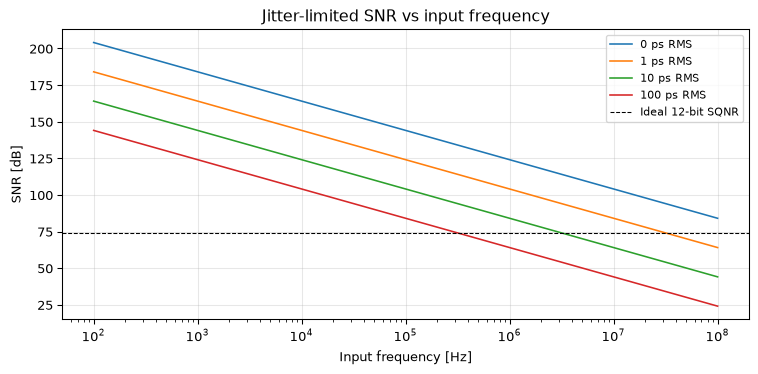
The sampling instant is never perfectly regular. Clock jitter in the ADC’s sample-and-hold causes the actual sampling time to vary by a random amount \(\sigma_j\) (RMS). For a sinusoidal input at frequency \(f_{in}\), the resulting voltage error is approximately \(2\pi f_{in} A \sigma_j\), giving
This is frequency-dependent: a 10 ps RMS jitter is inaudible at 1 kHz (SNR ≈ 144 dB) but limits a 100 MHz IF sampler to about 44 dB, barely 7 effective bits (\((44.0 - 1.76)/6.02 \approx 7.0\)), regardless of the ADC’s rated resolution.
Figure 1: Jitter-limited SNR vs input frequency. Each curve is a different RMS jitter value. High-frequency sampling demands picosecond-level clock stability.
INL/DNL: non-uniform steps
DNL (differential nonlinearity) is the deviation of each quantisation step from the ideal \(Q\). A DNL of ±0.5 LSB means some codes are wider, some narrower: the quantisation error is no longer uniform. INL (integral nonlinearity) is the cumulative deviation from the ideal transfer curve. INL creates harmonics because the error is signal-dependent; it is distortion, not noise, and it does not average out.
Thermal noise
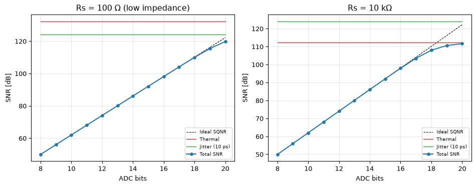
The ADC’s input sampling capacitor, the source resistance, and the amplifier front-end all contribute thermal (Johnson-Nyquist) noise. For a source resistance \(R_s\) at temperature \(T\), the RMS noise voltage over the Nyquist bandwidth \(f_s/2\) is
\[v_n = \sqrt{4 k_B T R_s \cdot f_s/2} \quad [\text{V}_\text{RMS}].\]
Figure 2: ADC noise budget: quantisation, thermal, and jitter components sum in quadrature. At 12 bits quantisation noise dominates for low source impedance. Past 18 bits thermal noise from a 10 k-ohm source becomes the limiting factor; at 16 bits the thermal contribution is only ~0.15 dB.
At high source impedance, thermal noise overtakes quantisation noise around 18 bits; at 14 bits the thermal contribution is negligible, but beyond 18 bits the front-end physics, not the converter resolution, sets the noise floor.
ENOB: the bits you actually get
The effective number of bits is computed from the measured SINAD (signal-to-noise-and-distortion ratio):
A 12-bit ADC with SINAD of 68 dB has ENOB ≈ 11.0: you lost a bit to noise and distortion. This is normal. A “12-bit” ADC with ENOB of 9.5 is either broken or being used outside its specified conditions (Kester 2005).
Oversampling: trading bandwidth for bits
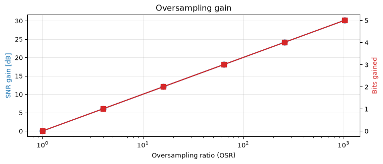
If the quantisation noise is white, oversampling by a factor OSR (the ratio of sample rate to twice the signal bandwidth) spreads the same total quantisation noise power over a wider bandwidth. A digital low-pass filter then removes the out-of-band noise, improving the in-band SNR by
Four times the sample rate buys 1 bit (6.02 dB). This only works if the noise is white: \(1/f\) noise or interference does not average as \(1/\sqrt{\text{OSR}}\).
Show the code
osr = np.array([1, 4, 16, 64, 256, 1024])gain = oversampling_gain(osr)bits_gained = gain /6.02fig, ax = plt.subplots(figsize=(8, 3.5))ax2 = ax.twinx()ax.semilogx(osr, gain, 'C0o-', markersize=8)ax2.semilogx(osr, bits_gained, 'C3s-', markersize=8)ax.set_xlabel('Oversampling ratio (OSR)'); ax.set_ylabel('SNR gain [dB]', color='C0')ax2.set_ylabel('Bits gained', color='C3')ax.set_title('Oversampling gain'); ax.grid(True, alpha=0.3)fig.tight_layout(); plt.show()for o, g, b inzip(osr, gain, bits_gained):print(f"OSR={o:4d}: gain={g:.1f} dB, bits gained={b:.1f}")
Figure 3: Oversampling gain: each 4× increase in OSR buys 6 dB (1 bit) for white quantisation noise.
Oversampling spreads the noise; noise shaping pushes it out of band. A sigma-delta modulator places the quantiser inside a feedback loop with a loop filter \(H(z)\). The quantisation noise experiences a high-pass transfer function \(\text{NTF}(z) = (1 - z^{-1})^L\), where \(L\) is the loop order. The in-band noise after decimation is dramatically reduced (Maloberti 2007):
A 1-bit (\(M = 1\)) second-order modulator at OSR = 256 gives an ideal SQNR of about 115 dB, equivalent to a 19-bit Nyquist converter, from a single comparator. (The ideal formula is optimistic; practical implementations with non-ideal integrators and clock jitter achieve somewhat less, which is why audio converters push OSR well into the hundreds.)
Inside the modulator
The formula above treats the modulator as a black box. The box is worth opening, because it is built from parts this site has already dissected. The first-order loop, in the form introduced by Inose, Yasuda and Murakami in 1962 (Inose, Yasuda, and Murakami 1962), is one accumulator and one comparator:
The accumulator integrates the difference between the input and the 1-bit output; the comparator feeds back the coarsest possible quantisation. Linearise the comparator as an additive error \(e[n]\) and the loop algebra gives
\[Y(z) = z^{-1}\,X(z) + (1 - z^{-1})\,E(z):\]
the signal passes with a pure delay (STF \(= z^{-1}\)), while the quantisation error is differentiated (NTF \(= 1 - z^{-1}\)). Every block here is a member of the integrator-comb family from the smoothing chapter(Lyons and Bell 2004): the forward path is the integrator \(1/(1-z^{-1})\), the noise sees the differentiator \(1-z^{-1}\), and the decimation filter that turns the bitstream back into multi-bit samples is the moving average / CIC built from the same two blocks. A second-order loop adds one more integrator (with the feedback weighted \(2y\) into the second stage) and squares the NTF to \((1-z^{-1})^2\).
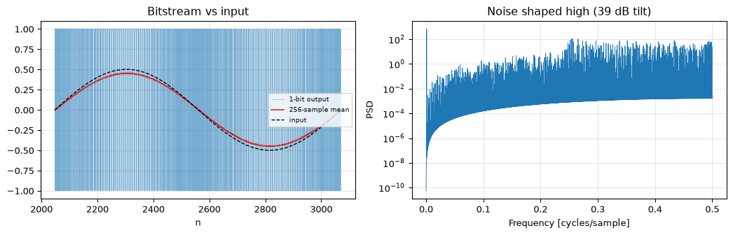
Run the actual loop, not the linearised model, and both claims are checkable:
Show the code
from adc_noise import sigma_delta_modulate, sigma_delta_decimatefrom scipy.signal import welchn =1<<16t = np.arange(n)f_sig =1/1024x =0.5* np.sin(2* np.pi * f_sig * t)bits = sigma_delta_modulate(x, order=1)# Self-check 1: the windowed bitstream mean must track the input.window =256local_mean = np.convolve(bits, np.ones(window) / window, mode='same')track_err = np.sqrt(np.mean((local_mean[window:-window] - x[window:-window])**2))assert track_err <0.05, f"bitstream average should track the input, RMS err {track_err:.3f}"# Self-check 2: the noise must be shaped high (differentiator tilt).f, psd = welch(bits, 1.0, nperseg=8192)sig_mask = np.abs(f - f_sig) <=3* (f[1] - f[0])tilt_db =10* np.log10(psd[f >0.4].mean() / psd[(f >0) & (f <0.01) &~sig_mask].mean())assert tilt_db >20, f"expected a strong low-to-high noise tilt, got {tilt_db:.1f} dB"fig, axes = plt.subplots(1, 2, figsize=(11, 3.6))zoom =slice(2048, 2048+1024)axes[0].step(t[zoom], bits[zoom], 'C0-', linewidth=0.4, alpha=0.6, label='1-bit output')axes[0].plot(t[zoom], local_mean[zoom], 'C3-', linewidth=1.2, label=f'{window}-sample mean')axes[0].plot(t[zoom], x[zoom], 'k--', linewidth=1.0, label='input')axes[0].set_xlabel('n'); axes[0].set_title('Bitstream vs input')axes[0].legend(fontsize=7); axes[0].grid(True, alpha=0.3)axes[1].semilogy(f, psd, 'C0-', linewidth=0.6)axes[1].set_xlabel('Frequency [cycles/sample]'); axes[1].set_ylabel('PSD')axes[1].set_title(f'Noise shaped high ({tilt_db:.0f} dB tilt)')axes[1].grid(True, alpha=0.3)fig.tight_layout(); plt.show()
Figure 4: First-order sigma-delta modulation of a slow sine. Left: the 1-bit output switches so that its short-window average (red) tracks the input (black). Right: the bitstream PSD shows the differentiator signature; the quantisation noise is pushed up and away from the signal at the far left.
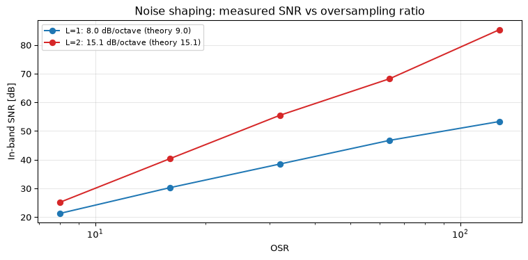
The measured in-band SNR follows the promised slope: roughly 9 dB per octave of OSR for first order, 15 dB per octave for second order.
Show the code
def inband_snr(bits, f_sig, osr, fs=1.0): f, psd = welch(bits, fs, nperseg=8192) band = f <= fs / (2* osr) sig = np.abs(f - f_sig) <=2* (f[1] - f[0])return10* np.log10(psd[sig & band].sum() / psd[band &~sig].sum())n2 =1<<17x2 =0.5* np.sin(2* np.pi * f_sig * np.arange(n2))# OSR capped at 128: at OSR 256 the integration band holds so few bins# beyond the excluded signal bins that the estimate becomes erratic.osrs = np.array([8, 16, 32, 64, 128])fig, ax = plt.subplots(figsize=(8, 4))theory_slope = {1: 30* np.log10(2), 2: 50* np.log10(2)} # 9.03, 15.05for order, color in [(1, 'C0'), (2, 'C3')]: b = sigma_delta_modulate(x2, order=order) snr = np.array([inband_snr(b, f_sig, o) for o in osrs]) per_octave = (snr[-1] - snr[0]) / np.log2(osrs[-1] / osrs[0])# Pin the caption's numbers: measured 8.0 (L=1) and 15.1 (L=2)# dB/octave, within 1.5 dB/octave of the ideal-formula slope.assertabs(per_octave - theory_slope[order]) <1.5, \f"L={order}: measured {per_octave:.1f} dB/octave vs theory {theory_slope[order]:.1f}" ax.semilogx(osrs, snr, f'{color}o-', label=f'L={order}: {per_octave:.1f} dB/octave (theory {theory_slope[order]:.1f})')ax.set_xlabel('OSR'); ax.set_ylabel('In-band SNR [dB]')ax.set_title('Noise shaping: measured SNR vs oversampling ratio')ax.legend(fontsize=8); ax.grid(True, alpha=0.3)fig.tight_layout(); plt.show()
Figure 5: Measured in-band SNR of the simulated modulators vs OSR. The ideal formula predicts slopes of 9.0 dB per octave (first order) and 15.1 dB per octave (second order); this simulation measures 8.0 and 15.1 over OSR 8 to 128. The absolute SNR sits below the ideal formula because the input is at half scale and the band-edge integration is conservative; the slopes are what the theory pins down.
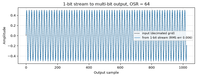
The final step of the pipeline is the one this site already covers: decimation. A moving-average (CIC-style) low-pass removes the shaped high-frequency noise and the downsampler returns to the Nyquist rate; multi-bit resolution reappears from a 1-bit stream.
Figure 6: Closing the loop: the 1-bit stream, filtered by a sinc-squared decimator (two cascaded moving averages) and downsampled by 64, reproduces the input waveform. One comparator plus averaging equals a multi-bit converter.
DDS phase truncation: the same trick on the phase path
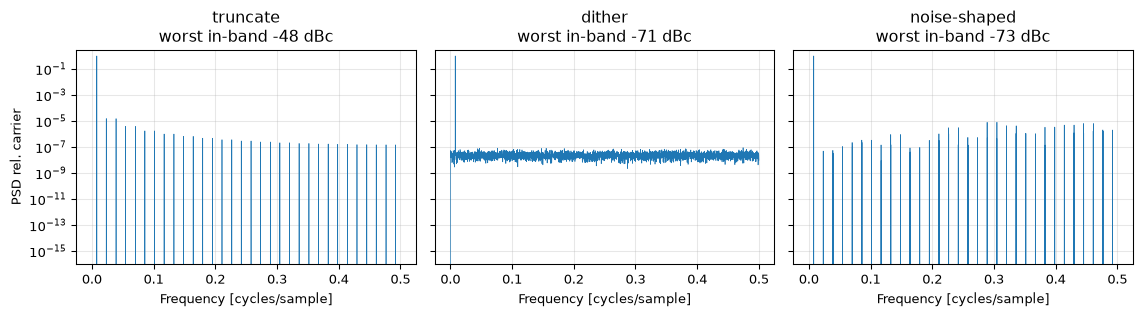
Noise shaping is not only for amplitude quantisers. In direct digital synthesis (DDS), a wide phase accumulator (say 24 or 32 bits) advances by a tuning word every sample and its top bits address a sine lookup table. The discarded low bits are a quantisation of phase, and because the accumulator sequence is periodic, that error is periodic too: it shows up as discrete spurs, not a noise floor. Nicholas and Samueli’s classical analysis (Nicholas and Samueli 1987) locates the spurs and bounds the worst one at close to \(-6.02\,W\) dBc for a \(W\)-bit table address.
The three standard treatments of the discarded bits are exactly the noise strategies of this arc: live with the spurs, dither them white, or noise-shape them out of band with the sigma-delta differentiator applied to the phase error (first-order error feedback: add the previous sample’s truncation residual back in before truncating).
Show the code
from adc_noise import dds_sinen_dds =1<<15nps =8192f_word = (1<<17) +2048# lands exactly on a Welch bin; low bits activef0 = f_word /2**24fig, axes = plt.subplots(1, 3, figsize=(12, 3.4), sharey=True)results = {}for ax, mode inzip(axes, ('truncate', 'dither', 'noise-shaped')): xd = dds_sine(n_dds, f_word, phase_bits=24, table_bits=8, mode=mode, seed=1) f, psd = welch(xd, 1.0, nperseg=nps, window='boxcar') sig = np.abs(f - f0) <=1.5* (f[1] - f[0]) carrier = psd[sig].max() rest_f, rest = f[~sig & (f >0)], psd[~sig & (f >0)] results[mode] = {'worst': 10* np.log10(rest.max() / carrier),'inband': 10* np.log10(rest[rest_f <0.05].max() / carrier), } ax.semilogy(f, psd / carrier, 'C0-', linewidth=0.5) ax.set_ylim(1e-16, 3) ax.set_title(f"{mode}\nworst in-band {results[mode]['inband']:.0f} dBc") ax.set_xlabel('Frequency [cycles/sample]') ax.grid(True, alpha=0.3)axes[0].set_ylabel('PSD rel. carrier')fig.tight_layout(); plt.show()# Self-checks: the caption's three claims, measured. The truncation spur# is pinned to the caption's -48 dBc (measured -48.1; the -6.02*8 rule# predicts -48.2), not a loose window.assert-50< results['truncate']['worst'] <-46, "truncation spur should sit at ~-48 dBc"assert results['dither']['worst'] <-65, "dither should bury the spurs"assert results['noise-shaped']['inband'] <-65, "error feedback should clear the band"assert results['noise-shaped']['worst'] > results['noise-shaped']['inband'] +10, \"the shaped error must sit out of band"
Figure 7: DDS output spectra with a 24-bit accumulator and an 8-bit table, for a worst-case-style tuning word. Truncation concentrates the phase error into in-band spurs at -48 dBc (the -6.02 dB/bit rule). Dither trades the spurs for a flat noise floor. First-order error feedback clears the low-frequency band and pushes the error toward Nyquist, where an output filter removes it.
On hardware the error-feedback shaper costs one addition and one AND-mask per sample, which is why it is standard in commercial DDS chips. The embedded companion builds the amplitude-domain equivalent: a 1-bit sigma-delta DAC on a GPIO pin.
Test yourself
A few checks that the formulas above are at your fingertips. Each is answerable with pencil and paper plus, if you want confirmation, sigma_delta_snr() from the module.
1 (basic). A first-order 1-bit sigma-delta modulator runs at OSR = 64. What is the ideal SQNR, and how many effective bits is that?
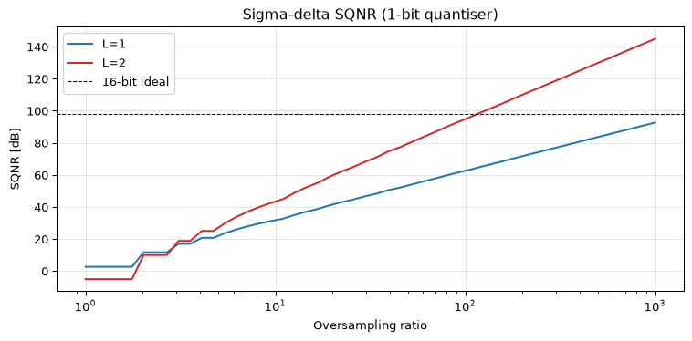
2 (intermediate). You need 16-bit audio quality (\(\text{SQNR} \geq 6.02 \cdot 16 + 1.76 = 98.1\) dB) from a 1-bit second-order modulator. What is the minimum power-of-two OSR? Check whether one octave lower would do.
Solution
Solve \(7.78 - 10\log_{10}(\pi^4/5) + 5 \cdot 10\log_{10}(\text{OSR}) \geq 98.1\) with \(10\log_{10}(\pi^4/5) = 12.90\): \(50\log_{10}(\text{OSR}) \geq 103.2\), so \(\text{OSR} \geq 116\), and the minimum power of two is 128 (100.2 dB). One octave lower, OSR = 64, gives only 85.2 dB and fails. (sigma_delta_snr(1, 128, order=2) = 100.2 dB, sigma_delta_snr(1, 64, order=2) = 85.2 dB.)
3 (challenge). A DDS uses a 32-bit phase accumulator and a 10-bit sine table, and your application needs all spurs below \(-80\) dBc in the band of interest. (a) Estimate the worst-case truncation spur. (b) One fix is a bigger table: how many address bits would you need, and what is the table-size cost? (c) Name the fix that keeps the 10-bit table, and its price.
Solution
Worst spur \(\approx -6.02 \cdot 10 \approx -60\) dBc: 20 dB short of the requirement.
You need \(W \geq 80/6.02 \approx 13.3\), so a 14-bit address: \(2^{14} = 16{,}384\) entries, a 16-fold table-size increase over \(2^{10} = 1{,}024\).
First-order error feedback on the truncated phase (or dither, if a raised flat floor is acceptable). Price: the phase error is pushed to high frequencies, so it must be removed downstream (the DAC’s reconstruction filter, or an oversampled band with margin), and near-Nyquist output frequencies get less protection. Dither instead trades the spurs for a raised flat noise floor across the whole band (in the 8-bit-table demo above, the dithered floor’s worst lines sat near \(-71\) dBc; a 10-bit table starts lower), which may or may not fit a spurious-free spec.
Show the code
osr_range = np.logspace(0, 3, 50)fig, ax = plt.subplots(figsize=(8, 4))for L, color in [(1, 'C0'), (2, 'C3')]: sqnr = [sigma_delta_snr(1, int(o), order=L) for o in osr_range] ax.semilogx(osr_range, sqnr, color=color, linewidth=1.5, label=f'L={L}')ax.axhline(6.02*16+1.76, color='k', linestyle='--', linewidth=0.8, label='16-bit ideal')ax.set_xlabel('Oversampling ratio'); ax.set_ylabel('SQNR [dB]')ax.set_title('Sigma-delta SQNR (1-bit quantiser)'); ax.legend(); ax.grid(True, alpha=0.3)fig.tight_layout(); plt.show()
Figure 8: Ideal sigma-delta SQNR vs oversampling ratio. Second-order shaping gives dramatically more bits per octave of oversampling than first-order.
Datasheet literacy: nV/√Hz, SFDR, SINAD
When reading an ADC datasheet, the key noise specs are:
Spec
What it tells you
Unit
Input-referred noise
Total noise referred to the input
μV RMS or nV/√Hz
SINAD
SNR + distortion together
dB
SFDR
Spurious-free dynamic range: the distance from the carrier to the largest spur
dBc
ENOB
Effective bits = (SINAD − 1.76)/6.02
bits
A common trap: the datasheet quotes SINAD at a low input frequency (e.g., 10 kHz) where jitter is negligible. At your actual operating frequency, jitter may dominate and the effective bits are much lower. Always check the SINAD vs frequency plot.
On hardware
Characterising the noise floor of a real STM32 ADC (measuring ENOB, identifying the limiting noise source, and verifying oversampling gain) is covered in the embedded companion.
Going further
PSD estimation: the tool for measuring ADC noise floors: Welch on the raw ADC output reveals jitter skirts, INL harmonics, and \(1/f\) noise that the datasheet single-number specs do not capture.
Finite word-length effects: what happens to a filter’s coefficients and arithmetic after the ADC delivers its bits.
Dither: adding noise before quantisation to linearise the transfer curve; the sigma-delta’s feedback loop is a noise-shaping extension of the dither principle.
References
Inose, Hiroshi, Yasuhiko Yasuda, and J. Murakami. 1962. “A Telemetering System by Code Modulation: Delta-Sigma Modulation.”IRE Transactions on Space Electronics and Telemetry 8: 204–9.
Kester, Walt. 2005. The Data Conversion Handbook. Analog Devices / Newnes.
Lyons, Richard G., and Amy E. Bell. 2004. “The Swiss Army Knife of Digital Networks.”IEEE Signal Processing Magazine 21 (3): 90–100.
Maloberti, Franco. 2007. Data Converters. Springer.
Nicholas, Henry T., and Henry Samueli. 1987. “An Analysis of the Output Spectrum of Direct Digital Frequency Synthesizers in the Presence of Phase-Accumulator Truncation.” In Proceedings of the 41st Annual Frequency Control Symposium, 495–502.
Source Code
---title: "ADC Noise"subtitle: "The noise sources that eat your effective bits"description-meta: "Why a real converter never reaches 6.02B + 1.76 dB: jitter, thermal noise and nonlinearity, and what each one costs in effective bits."bibliography: ../../references.bib---The [basics chapter](../../basics/03-noise-snr.qmd) gives the headline: a $B$-bit ADC has $\text{SQNR} = 6.02B + 1.76$ dB. That formula assumes an ideal converter: perfect sampling instants, exactly equal steps, and no noise except quantisation. Real ADCs have all three, and each one eats effective bits.This page models the major non-ideal noise sources, shows how to compute the effective number of bits (ENOB) from datasheet specs or measured data, and explains how oversampling and noise shaping buy bits back. The [embedded companion](embedded.qmd) takes it to the metal: characterising the noise floor of a real STM32 ADC.::: {.callout-note title="Prerequisites"}Part of the [noise & stochastic processing arc](../noise-and-stochastic-processing.qmd); the overview gives the reading order.[Noise and SNR](../../basics/03-noise-snr.qmd) (quantisation SNR), [random processes](../random-processes/index.qmd) (thermal and jitter as random processes), and [PSD estimation](../psd-estimation/index.qmd) (how to measure the noise floor).:::::: {.callout-tip title="Code"}The implementation is [`adc_noise.py`](adc_noise.py). Save [`test_adc_noise.py`](test_adc_noise.py) beside it and `pytest test_adc_noise.py` runs the checks on it.:::```{python}#| echo: falseimport numpy as npimport matplotlib.pyplot as pltfrom adc_noise import (jitter_snr, enob_from_sinad, oversampling_gain, sigma_delta_snr, adc_noise_budget)```<hr>## The three noise sources beyond quantisation### Aperture jitterThe sampling instant is never perfectly regular. Clock jitter in the ADC's sample-and-hold causes the actual sampling time to vary by a random amount $\sigma_j$ (RMS). For a sinusoidal input at frequency $f_{in}$, the resulting voltage error is approximately $2\pi f_{in} A \sigma_j$, giving$$\text{SNR}_\text{jitter} = -20\log_{10}(2\pi f_{in} \sigma_j) \quad [\text{dB}].$$This is frequency-dependent: a 10 ps RMS jitter is inaudible at 1 kHz (SNR ≈ 144 dB) but limits a 100 MHz IF sampler to about 44 dB, barely 7 effective bits ($(44.0 - 1.76)/6.02 \approx 7.0$), regardless of the ADC's rated resolution.```{python}#| label: fig-jitter#| fig-cap: "Jitter-limited SNR vs input frequency. Each curve is a different RMS jitter value. High-frequency sampling demands picosecond-level clock stability."f_in = np.logspace(2, 8, 200) # 100 Hz to 100 MHzjitters = [100e-15, 1e-12, 10e-12, 100e-12]fig, ax = plt.subplots(figsize=(8, 4))for sj in jitters: snr = jitter_snr(f_in, sj) ax.semilogx(f_in, snr, linewidth=1.2, label=f'{sj*1e12:.0f} ps RMS')ax.axhline(6.02*12+1.76, color='k', linestyle='--', linewidth=0.8, label='Ideal 12-bit SQNR')ax.set_xlabel('Input frequency [Hz]'); ax.set_ylabel('SNR [dB]')ax.set_title('Jitter-limited SNR vs input frequency')ax.legend(fontsize=8); ax.grid(True, alpha=0.3)fig.tight_layout(); plt.show()```### INL/DNL: non-uniform steps**DNL** (differential nonlinearity) is the deviation of each quantisation step from the ideal $Q$. A DNL of ±0.5 LSB means some codes are wider, some narrower: the quantisation error is no longer uniform. **INL** (integral nonlinearity) is the cumulative deviation from the ideal transfer curve. INL creates harmonics because the error is signal-dependent; it is distortion, not noise, and it does not average out.### Thermal noiseThe ADC's input sampling capacitor, the source resistance, and the amplifier front-end all contribute thermal (Johnson-Nyquist) noise. For a source resistance $R_s$ at temperature $T$, the RMS noise voltage over the Nyquist bandwidth $f_s/2$ is$$v_n = \sqrt{4 k_B T R_s \cdot f_s/2} \quad [\text{V}_\text{RMS}].$$```{python}#| label: fig-noise-budget#| fig-cap: "ADC noise budget: quantisation, thermal, and jitter components sum in quadrature. At 12 bits quantisation noise dominates for low source impedance. Past 18 bits thermal noise from a 10 k-ohm source becomes the limiting factor; at 16 bits the thermal contribution is only ~0.15 dB."bits_range = np.arange(8, 21)fs =100e3f_in =10e3fig, axes = plt.subplots(1, 2, figsize=(10, 4))for ax, R_source, title inzip(axes, [100.0, 10000.0], ['Rs = 100 Ω (low impedance)', 'Rs = 10 kΩ']): sqnr_ideal = []; thermal = []; jitter = []; total = []for b in bits_range: bud = adc_noise_budget(bits=b, fs=fs, f_in=f_in, R_source=R_source, T=293.0, sigma_jitter=10e-12) sqnr_ideal.append(bud['sqnr_ideal']) thermal.append(bud['thermal_snr']) jitter.append(bud['jitter_snr']) total.append(bud['total_snr']) ax.plot(bits_range, sqnr_ideal, 'k--', linewidth=0.8, label='Ideal SQNR') ax.plot(bits_range, thermal, 'C3-', linewidth=1, label='Thermal') ax.plot(bits_range, jitter, 'C2-', linewidth=1, label='Jitter (10 ps)') ax.plot(bits_range, total, 'C0o-', linewidth=1.5, markersize=4, label='Total SNR') ax.set_xlabel('ADC bits'); ax.set_ylabel('SNR [dB]') ax.set_title(title); ax.legend(fontsize=7); ax.grid(True, alpha=0.3)fig.tight_layout(); plt.show()```At high source impedance, thermal noise overtakes quantisation noise around 18 bits; at 14 bits the thermal contribution is negligible, but beyond 18 bits the front-end physics, not the converter resolution, sets the noise floor.<hr>## ENOB: the bits you actually getThe effective number of bits is computed from the measured SINAD (signal-to-noise-and-distortion ratio):$$\text{ENOB} = \frac{\text{SINAD}_\text{dB} - 1.76}{6.02}.$$A 12-bit ADC with SINAD of 68 dB has ENOB ≈ 11.0: you lost a bit to noise and distortion. This is normal. A "12-bit" ADC with ENOB of 9.5 is either broken or being used outside its specified conditions [@kester2005data].<hr>## Oversampling: trading bandwidth for bitsIf the quantisation noise is white, oversampling by a factor OSR (the ratio of sample rate to twice the signal bandwidth) spreads the same total quantisation noise power over a wider bandwidth. A digital low-pass filter then removes the out-of-band noise, improving the in-band SNR by$$\Delta\text{SNR} = 10\log_{10}(\text{OSR}) \quad [\text{dB}].$$Four times the sample rate buys 1 bit (6.02 dB). This only works if the noise is white: $1/f$ noise or interference does not average as $1/\sqrt{\text{OSR}}$.```{python}#| label: fig-oversampling#| fig-cap: "Oversampling gain: each 4× increase in OSR buys 6 dB (1 bit) for white quantisation noise."osr = np.array([1, 4, 16, 64, 256, 1024])gain = oversampling_gain(osr)bits_gained = gain /6.02fig, ax = plt.subplots(figsize=(8, 3.5))ax2 = ax.twinx()ax.semilogx(osr, gain, 'C0o-', markersize=8)ax2.semilogx(osr, bits_gained, 'C3s-', markersize=8)ax.set_xlabel('Oversampling ratio (OSR)'); ax.set_ylabel('SNR gain [dB]', color='C0')ax2.set_ylabel('Bits gained', color='C3')ax.set_title('Oversampling gain'); ax.grid(True, alpha=0.3)fig.tight_layout(); plt.show()for o, g, b inzip(osr, gain, bits_gained):print(f"OSR={o:4d}: gain={g:.1f} dB, bits gained={b:.1f}")```<hr>## Noise shaping: sigma-delta conversionOversampling spreads the noise; **noise shaping** pushes it out of band. A sigma-delta modulator places the quantiser inside a feedback loop with a loop filter $H(z)$. The quantisation noise experiences a high-pass transfer function $\text{NTF}(z) = (1 - z^{-1})^L$, where $L$ is the loop order. The in-band noise after decimation is dramatically reduced [@maloberti2007converters]:$$\text{SQNR} \approx 6.02M + 1.76 - 10\log_{10}\frac{\pi^{2L}}{2L+1} + (2L+1)\cdot 10\log_{10}(\text{OSR}).$$A 1-bit ($M = 1$) second-order modulator at OSR = 256 gives an ideal SQNR of about 115 dB, equivalent to a 19-bit Nyquist converter, from a single comparator. (The ideal formula is optimistic; practical implementations with non-ideal integrators and clock jitter achieve somewhat less, which is why audio converters push OSR well into the hundreds.)### Inside the modulatorThe formula above treats the modulator as a black box. The box is worth opening, because it is built from parts this site has already dissected. The first-order loop, in the form introduced by Inose, Yasuda and Murakami in 1962 [@inose1962telemetering], is one accumulator and one comparator:$$y[n] = \operatorname{sign}(s[n]), \qquad s[n+1] = s[n] + x[n] - y[n].$$The accumulator integrates the difference between the input and the 1-bit output; the comparator feeds back the coarsest possible quantisation. Linearise the comparator as an additive error $e[n]$ and the loop algebra gives$$Y(z) = z^{-1}\,X(z) + (1 - z^{-1})\,E(z):$$the signal passes with a pure delay (STF $= z^{-1}$), while the quantisation error is *differentiated* (NTF $= 1 - z^{-1}$). Every block here is a member of the integrator-comb family from the [smoothing chapter](../../basics/08-smoothing/index.qmd#direct-vs-recursive-implementation)[@lyons2004swissarmy]: the forward path is the integrator $1/(1-z^{-1})$, the noise sees the differentiator $1-z^{-1}$, and the decimation filter that turns the bitstream back into multi-bit samples is the moving average / [CIC](../../basics/10-multirate/index.qmd) built from the same two blocks. A second-order loop adds one more integrator (with the feedback weighted $2y$ into the second stage) and squares the NTF to $(1-z^{-1})^2$.Run the actual loop, not the linearised model, and both claims are checkable:```{python}#| label: fig-sd-bitstream#| fig-cap: "First-order sigma-delta modulation of a slow sine. Left: the 1-bit output switches so that its short-window average (red) tracks the input (black). Right: the bitstream PSD shows the differentiator signature; the quantisation noise is pushed up and away from the signal at the far left."from adc_noise import sigma_delta_modulate, sigma_delta_decimatefrom scipy.signal import welchn =1<<16t = np.arange(n)f_sig =1/1024x =0.5* np.sin(2* np.pi * f_sig * t)bits = sigma_delta_modulate(x, order=1)# Self-check 1: the windowed bitstream mean must track the input.window =256local_mean = np.convolve(bits, np.ones(window) / window, mode='same')track_err = np.sqrt(np.mean((local_mean[window:-window] - x[window:-window])**2))assert track_err <0.05, f"bitstream average should track the input, RMS err {track_err:.3f}"# Self-check 2: the noise must be shaped high (differentiator tilt).f, psd = welch(bits, 1.0, nperseg=8192)sig_mask = np.abs(f - f_sig) <=3* (f[1] - f[0])tilt_db =10* np.log10(psd[f >0.4].mean() / psd[(f >0) & (f <0.01) &~sig_mask].mean())assert tilt_db >20, f"expected a strong low-to-high noise tilt, got {tilt_db:.1f} dB"fig, axes = plt.subplots(1, 2, figsize=(11, 3.6))zoom =slice(2048, 2048+1024)axes[0].step(t[zoom], bits[zoom], 'C0-', linewidth=0.4, alpha=0.6, label='1-bit output')axes[0].plot(t[zoom], local_mean[zoom], 'C3-', linewidth=1.2, label=f'{window}-sample mean')axes[0].plot(t[zoom], x[zoom], 'k--', linewidth=1.0, label='input')axes[0].set_xlabel('n'); axes[0].set_title('Bitstream vs input')axes[0].legend(fontsize=7); axes[0].grid(True, alpha=0.3)axes[1].semilogy(f, psd, 'C0-', linewidth=0.6)axes[1].set_xlabel('Frequency [cycles/sample]'); axes[1].set_ylabel('PSD')axes[1].set_title(f'Noise shaped high ({tilt_db:.0f} dB tilt)')axes[1].grid(True, alpha=0.3)fig.tight_layout(); plt.show()```The measured in-band SNR follows the promised slope: roughly 9 dB per octave of OSR for first order, 15 dB per octave for second order.```{python}#| label: fig-sd-osr#| fig-cap: "Measured in-band SNR of the simulated modulators vs OSR. The ideal formula predicts slopes of 9.0 dB per octave (first order) and 15.1 dB per octave (second order); this simulation measures 8.0 and 15.1 over OSR 8 to 128. The absolute SNR sits below the ideal formula because the input is at half scale and the band-edge integration is conservative; the slopes are what the theory pins down."def inband_snr(bits, f_sig, osr, fs=1.0): f, psd = welch(bits, fs, nperseg=8192) band = f <= fs / (2* osr) sig = np.abs(f - f_sig) <=2* (f[1] - f[0])return10* np.log10(psd[sig & band].sum() / psd[band &~sig].sum())n2 =1<<17x2 =0.5* np.sin(2* np.pi * f_sig * np.arange(n2))# OSR capped at 128: at OSR 256 the integration band holds so few bins# beyond the excluded signal bins that the estimate becomes erratic.osrs = np.array([8, 16, 32, 64, 128])fig, ax = plt.subplots(figsize=(8, 4))theory_slope = {1: 30* np.log10(2), 2: 50* np.log10(2)} # 9.03, 15.05for order, color in [(1, 'C0'), (2, 'C3')]: b = sigma_delta_modulate(x2, order=order) snr = np.array([inband_snr(b, f_sig, o) for o in osrs]) per_octave = (snr[-1] - snr[0]) / np.log2(osrs[-1] / osrs[0])# Pin the caption's numbers: measured 8.0 (L=1) and 15.1 (L=2)# dB/octave, within 1.5 dB/octave of the ideal-formula slope.assertabs(per_octave - theory_slope[order]) <1.5, \f"L={order}: measured {per_octave:.1f} dB/octave vs theory {theory_slope[order]:.1f}" ax.semilogx(osrs, snr, f'{color}o-', label=f'L={order}: {per_octave:.1f} dB/octave (theory {theory_slope[order]:.1f})')ax.set_xlabel('OSR'); ax.set_ylabel('In-band SNR [dB]')ax.set_title('Noise shaping: measured SNR vs oversampling ratio')ax.legend(fontsize=8); ax.grid(True, alpha=0.3)fig.tight_layout(); plt.show()```The final step of the pipeline is the one this site already covers: decimation. A moving-average (CIC-style) low-pass removes the shaped high-frequency noise and the downsampler returns to the Nyquist rate; multi-bit resolution reappears from a 1-bit stream.```{python}#| label: fig-sd-decimate#| fig-cap: "Closing the loop: the 1-bit stream, filtered by a sinc-squared decimator (two cascaded moving averages) and downsampled by 64, reproduces the input waveform. One comparator plus averaging equals a multi-bit converter."osr =64y_dec = sigma_delta_decimate(bits, osr)ref = x[::osr]rms = np.sqrt(np.mean((y_dec[4:-4] - ref[4:-4])**2))assert rms <0.02, f"decimated output should match the input, RMS {rms:.4f}"fig, ax = plt.subplots(figsize=(8, 3.2))ax.plot(ref, 'k--', linewidth=1.0, label='input (decimated grid)')ax.plot(y_dec, 'C0-', linewidth=1.0, label=f'from 1-bit stream (RMS err {rms:.3f})')ax.set_xlabel('Output sample'); ax.set_ylabel('Amplitude')ax.set_title(f'1-bit stream to multi-bit output, OSR = {osr}')ax.legend(fontsize=8); ax.grid(True, alpha=0.3)fig.tight_layout(); plt.show()```### DDS phase truncation: the same trick on the phase pathNoise shaping is not only for amplitude quantisers. In **direct digital synthesis** (DDS), a wide phase accumulator (say 24 or 32 bits) advances by a tuning word every sample and its top bits address a sine lookup table. The discarded low bits are a quantisation of *phase*, and because the accumulator sequence is periodic, that error is periodic too: it shows up as discrete **spurs**, not a noise floor. Nicholas and Samueli's classical analysis [@nicholas1987analysis] locates the spurs and bounds the worst one at close to $-6.02\,W$ dBc for a $W$-bit table address.The three standard treatments of the discarded bits are exactly the noise strategies of this arc: live with the spurs, [dither](../dither/index.qmd) them white, or noise-shape them out of band with the sigma-delta differentiator applied to the phase error (first-order error feedback: add the previous sample's truncation residual back in before truncating).```{python}#| label: fig-dds-spurs#| fig-cap: "DDS output spectra with a 24-bit accumulator and an 8-bit table, for a worst-case-style tuning word. Truncation concentrates the phase error into in-band spurs at -48 dBc (the -6.02 dB/bit rule). Dither trades the spurs for a flat noise floor. First-order error feedback clears the low-frequency band and pushes the error toward Nyquist, where an output filter removes it."from adc_noise import dds_sinen_dds =1<<15nps =8192f_word = (1<<17) +2048# lands exactly on a Welch bin; low bits activef0 = f_word /2**24fig, axes = plt.subplots(1, 3, figsize=(12, 3.4), sharey=True)results = {}for ax, mode inzip(axes, ('truncate', 'dither', 'noise-shaped')): xd = dds_sine(n_dds, f_word, phase_bits=24, table_bits=8, mode=mode, seed=1) f, psd = welch(xd, 1.0, nperseg=nps, window='boxcar') sig = np.abs(f - f0) <=1.5* (f[1] - f[0]) carrier = psd[sig].max() rest_f, rest = f[~sig & (f >0)], psd[~sig & (f >0)] results[mode] = {'worst': 10* np.log10(rest.max() / carrier),'inband': 10* np.log10(rest[rest_f <0.05].max() / carrier), } ax.semilogy(f, psd / carrier, 'C0-', linewidth=0.5) ax.set_ylim(1e-16, 3) ax.set_title(f"{mode}\nworst in-band {results[mode]['inband']:.0f} dBc") ax.set_xlabel('Frequency [cycles/sample]') ax.grid(True, alpha=0.3)axes[0].set_ylabel('PSD rel. carrier')fig.tight_layout(); plt.show()# Self-checks: the caption's three claims, measured. The truncation spur# is pinned to the caption's -48 dBc (measured -48.1; the -6.02*8 rule# predicts -48.2), not a loose window.assert-50< results['truncate']['worst'] <-46, "truncation spur should sit at ~-48 dBc"assert results['dither']['worst'] <-65, "dither should bury the spurs"assert results['noise-shaped']['inband'] <-65, "error feedback should clear the band"assert results['noise-shaped']['worst'] > results['noise-shaped']['inband'] +10, \"the shaped error must sit out of band"```On hardware the error-feedback shaper costs one addition and one AND-mask per sample, which is why it is standard in commercial DDS chips. The [embedded companion](embedded.qmd#sigma-delta-dac) builds the amplitude-domain equivalent: a 1-bit sigma-delta DAC on a GPIO pin.### Test yourself {#test-yourself}A few checks that the formulas above are at your fingertips. Each is answerable with pencil and paper plus, if you want confirmation, `sigma_delta_snr()` from the module.**1 (basic).** A first-order 1-bit sigma-delta modulator runs at OSR = 64. What is the ideal SQNR, and how many effective bits is that?::: {.callout-note collapse="true" title="Solution"}$\text{SQNR} = 6.02 + 1.76 - 10\log_{10}(\pi^2/3) + 3 \cdot 10\log_{10}(64) = 7.78 - 5.17 + 54.19 \approx 56.8$ dB.$\text{ENOB} = (56.8 - 1.76)/6.02 \approx 9.1$ bits: a comparator plus averaging delivers nine-plus bits. `sigma_delta_snr(1, 64, order=1)` returns 56.79 dB.:::**2 (intermediate).** You need 16-bit audio quality ($\text{SQNR} \geq 6.02 \cdot 16 + 1.76 = 98.1$ dB) from a 1-bit *second-order* modulator. What is the minimum power-of-two OSR? Check whether one octave lower would do.::: {.callout-note collapse="true" title="Solution"}Solve $7.78 - 10\log_{10}(\pi^4/5) + 5 \cdot 10\log_{10}(\text{OSR}) \geq 98.1$ with $10\log_{10}(\pi^4/5) = 12.90$: $50\log_{10}(\text{OSR}) \geq 103.2$, so $\text{OSR} \geq 116$, and the minimum power of two is **128** (100.2 dB). One octave lower, OSR = 64, gives only 85.2 dB and fails. (`sigma_delta_snr(1, 128, order=2)` = 100.2 dB, `sigma_delta_snr(1, 64, order=2)` = 85.2 dB.):::**3 (challenge).** A DDS uses a 32-bit phase accumulator and a 10-bit sine table, and your application needs all spurs below $-80$ dBc in the band of interest. (a) Estimate the worst-case truncation spur. (b) One fix is a bigger table: how many address bits would you need, and what is the table-size cost? (c) Name the fix that keeps the 10-bit table, and its price.::: {.callout-note collapse="true" title="Solution"}(a) Worst spur $\approx -6.02 \cdot 10 \approx -60$ dBc: 20 dB short of the requirement.(b) You need $W \geq 80/6.02 \approx 13.3$, so a 14-bit address: $2^{14} = 16{,}384$ entries, a **16-fold** table-size increase over $2^{10} = 1{,}024$.(c) First-order error feedback on the truncated phase (or dither, if a raised flat floor is acceptable). Price: the phase error is pushed to high frequencies, so it must be removed downstream (the DAC's reconstruction filter, or an oversampled band with margin), and near-Nyquist output frequencies get less protection. Dither instead trades the spurs for a raised flat noise floor across the whole band (in the 8-bit-table demo above, the dithered floor's worst lines sat near $-71$ dBc; a 10-bit table starts lower), which may or may not fit a spurious-free spec.:::```{python}#| label: fig-sigma-delta#| fig-cap: "Ideal sigma-delta SQNR vs oversampling ratio. Second-order shaping gives dramatically more bits per octave of oversampling than first-order."osr_range = np.logspace(0, 3, 50)fig, ax = plt.subplots(figsize=(8, 4))for L, color in [(1, 'C0'), (2, 'C3')]: sqnr = [sigma_delta_snr(1, int(o), order=L) for o in osr_range] ax.semilogx(osr_range, sqnr, color=color, linewidth=1.5, label=f'L={L}')ax.axhline(6.02*16+1.76, color='k', linestyle='--', linewidth=0.8, label='16-bit ideal')ax.set_xlabel('Oversampling ratio'); ax.set_ylabel('SQNR [dB]')ax.set_title('Sigma-delta SQNR (1-bit quantiser)'); ax.legend(); ax.grid(True, alpha=0.3)fig.tight_layout(); plt.show()```<hr>## Datasheet literacy: nV/√Hz, SFDR, SINADWhen reading an ADC datasheet, the key noise specs are:| Spec | What it tells you | Unit ||---|---|---|| Input-referred noise | Total noise referred to the input | μV RMS or nV/√Hz || SINAD | SNR + distortion together | dB || SFDR | Spurious-free dynamic range: the distance from the carrier to the largest spur | dBc || ENOB | Effective bits = (SINAD − 1.76)/6.02 | bits |A common trap: the datasheet quotes SINAD at a low input frequency (e.g., 10 kHz) where jitter is negligible. At your actual operating frequency, jitter may dominate and the effective bits are much lower. Always check the SINAD vs frequency plot.<hr>## On hardwareCharacterising the noise floor of a real STM32 ADC (measuring ENOB, identifying the limiting noise source, and verifying oversampling gain) is covered in the [embedded companion](embedded.qmd).<hr>## Going further- **[PSD estimation](../psd-estimation/index.qmd)**: the tool for measuring ADC noise floors: Welch on the raw ADC output reveals jitter skirts, INL harmonics, and $1/f$ noise that the datasheet single-number specs do not capture.- **[Finite word-length effects](../finite-wordlength/index.qmd)**: what happens to a filter's coefficients and arithmetic after the ADC delivers its bits.- **[Dither](../dither/index.qmd)**: adding noise before quantisation to linearise the transfer curve; the sigma-delta's feedback loop is a noise-shaping extension of the dither principle.## References::: {#refs}:::