Measuring microvolts under a mountain of 1/f noise
Some measurements are small and slow. The optical absorption of a blood sample, the resistance change of a strain gauge, the thermal signal of an infrared detector: quantities that change over seconds or not at all, buried in electronics whose noise grows without bound exactly where slow signals live. Averaging, the universal remedy of estimation basics, quietly stops working there, and it does not warn you.
The lock-in amplifier is the classic instrument built around the escape route (Meade 1983): move the measurement. Modulate the physical quantity up to a carrier frequency where the front end is quiet, measure the carrier’s amplitude, and you inherit the clean white-noise averaging law no matter what the noise does at DC. The previous page already built the measuring device without saying so: the coherent single-bin DFT is the digital lock-in. This page is about the strategy wrapped around it: why 1/f noise forces you up in frequency, what integration time buys and at what bandwidth cost, and what it means to run one against real hardware (the embedded companion builds an LED photometer from it).
The implementation is lockin.py. Save test_lockin.py beside it and pytest test_lockin.py runs the checks on it.
The enemy: a noise floor that is not flat
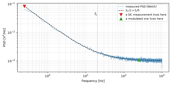
Every amplifier, every resistor, every ADC delivers a noise spectrum with the same general shape: a flat (white) floor at high frequencies, and a rise toward DC, usually close to \(1/f\), from slow processes in the components themselves: carrier trapping in transistors, temperature drift, ageing (Ward and Greenwood 2007). The two meet at the corner frequency\(f_c\), anywhere from millihertz for a good instrumentation amplifier to kilohertz for a cheap op-amp. Throughout this page the noise model is
\[S(f) = S_w\left(1 + \frac{f_c}{f}\right)\]
with \(S_w\) the one-sided white floor in \(\text{V}^2/\text{Hz}\). Below \(f_c\) the spectrum climbs without limit; a DC measurement sits at the bottom of that climb, at the worst point on the entire axis.
Figure 1: The front-end noise model, measured from a generated record (fs = 2 kHz, corner at 20 Hz) against the analytic S(f). A slow signal measured at baseband competes with the 1/f mountain; the same signal modulated to 250 Hz competes only with the white floor. The vertical distance between the two markers is the whole argument of this page.
Watching averaging fail
What does that mountain do to a measurement? Take the simplest possible task: estimate a constant level by averaging \(T\) seconds of data. In white noise the answer is on the estimation-basics page: variance \(\sigma^2/N\), so the error falls as \(1/\sqrt{T}\), forever. In \(1/f\) noise it does not.
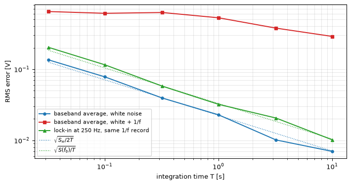
The mechanism is worth seeing without equations first. Averaging longer helps against noise that is faster than your averaging window, because fast wiggles cancel. But \(1/f\) noise has ever more power at ever slower time scales: stretch the window and you admit new, slower drift that was invisible before. The two effects nearly cancel, and the error curve goes flat. More data stops buying accuracy: not slowly, not eventually, but at a wall a little past \(1/f_c\) seconds.
Show the code
rng = np.random.default_rng(7)n_tot =2**21# ~17 minutes at 2 kHzxw = sigma_w * rng.standard_normal(n_tot)xp = front_end_noise(n_tot, sigma_w, corner, fs=fs, rng=rng)Ts = np.array([0.032, 0.1, 0.32, 1.0, 3.2, 10.0])f0 =250.0rms_w, rms_p, rms_l = [], [], []for T in Ts: nblk =int(round(T * fs)) nb =min(n_tot // nblk, 96) blk =lambda x: x[:nb * nblk].reshape(nb, nblk) rms_w.append(np.sqrt(np.mean(blk(xw).mean(axis=1)**2))) rms_p.append(np.sqrt(np.mean(blk(xp).mean(axis=1)**2)))# Lock-in: a unit-amplitude carrier on an exact bin of each block,# demodulated per block; the error is the amplitude misread. k =round(f0 * nblk / fs) f0b = k * fs / nblk tone = np.cos(2* np.pi * f0b * np.arange(nblk) / fs +0.3) errs = [lockin_block(seg + tone, f0b, fs=fs)[0] -1.0for seg in blk(xp)] rms_l.append(np.sqrt(np.mean(np.square(errs))))rms_w, rms_p, rms_l =map(np.array, (rms_w, rms_p, rms_l))S1_f0 = S_w * (1+ corner / f0)fig, ax = plt.subplots(figsize=(7.5, 4))ax.loglog(Ts, rms_w, 'o-C0', ms=4, label='baseband average, white noise')ax.loglog(Ts, rms_p, 's-C3', ms=4, label='baseband average, white + 1/f')ax.loglog(Ts, rms_l, '^-C2', ms=4, label='lock-in at 250 Hz, same 1/f record')ax.loglog(Ts, np.sqrt(S_w / (2* Ts)), 'C0:', lw=1, label=r'$\sqrt{S_w/2T}$')ax.loglog(Ts, np.sqrt(S1_f0 / Ts), 'C2:', lw=1, label=r'$\sqrt{S(f_0)/T}$')ax.set_xlabel('integration time T [s]'); ax.set_ylabel('RMS error [V]')ax.legend(fontsize=8); ax.grid(True, which='both', alpha=0.3)fig.tight_layout(); plt.show()gain_w = rms_w[0] / rms_w[-1]gain_p = rms_p[0] / rms_p[-1]gain_l = rms_l[0] / rms_l[-1]print(f"312x more data: white baseband {gain_w:.1f}x better, "f"1/f baseband {gain_p:.1f}x, lock-in {gain_l:.1f}x "f"(sqrt(312) = {np.sqrt(Ts[-1]/Ts[0]):.1f})")# White baseband must sit on sqrt(S_w/2T) throughout (the DC-level# bound has a factor 2: see the callout below).assert np.all(np.abs(rms_w / np.sqrt(S_w / (2* Ts)) -1) <0.2)# The wall: 1/f baseband improves by far less than sqrt(312) = 17.7.assert gain_p <3.0, "1/f averaging should hit a wall"assert gain_w >12.0, "white averaging should not"# The lock-in recovers the white law ON THE SAME 1/f RECORD.assert np.all((rms_l / np.sqrt(S1_f0 / Ts) >0.75)& (rms_l / np.sqrt(S1_f0 / Ts) <1.3))assert gain_l >12.0, "the lock-in should keep improving"
Figure 2: RMS error of a T-second average, measured over many disjoint blocks of one long record (fs = 2 kHz). In white noise (blue) the error falls as the promised T^(-1/2) across the whole sweep. In white + 1/f noise (red) the same estimator hits a wall near 1/f_c = 50 ms and a 300-fold increase in data buys almost nothing. The lock-in (green) measures the same record at a 250 Hz carrier instead, and recovers the white-noise law: its error keeps falling on the S(f0)/T line, three decades after the baseband curve has stopped.
312x more data: white baseband 19.3x better, 1/f baseband 2.2x, lock-in 19.9x (sqrt(312) = 17.7)
This is the plot that justifies everything else here. The red curve is not a badly built estimator; it is the best linear estimator for the job it was given, and the job is unwinnable. The green curve is the same record, the same total data, with the measurement moved 250 Hz up the spectrum first.
The fix: modulate up, demodulate down
So the strategy is: make the physical quantity ride a carrier. Chop the light with the LED drive, excite the bridge with an AC reference, vibrate the sample. If the measurand is \(m\) and the excitation is a carrier at \(f_0\), the front end now delivers
\[x(t) = \underbrace{G\, m \cos(2\pi f_0 t + \phi)}_{\text{signal, parked at } f_0} + \; w(t)\]
and estimating \(m\) means estimating the amplitude of a tone of known frequency, which is a solved problem: the coherent single-bin DFT from the previous page, which correlates the record with quadrature references at \(f_0\) and reads amplitude and phase off the complex result. A lock-in amplifier is that inner product, plus the modulation strategy, plus a low-pass filter to let you watch the amplitude move. lockin_block in this topic’s module is coherent_dft with a different hat on; the Goertzel filter is the same inner product computed recursively.
Nature’s version of carrying your own carrier
Supplying your own excitation so the measurement lands where you want it is a sensing strategy weakly electric fish arrived at first. The fish continuously emits an electric organ discharge, and nearby objects change the discharge-driven current at electroreceptors in its skin according to their conductivity, so what the receptors read is a modulation of the animal’s own transmitted carrier rather than any field the environment happened to provide (Emde 1999). The same fish appears on the adaptive-filtering page for a different trick entirely: shifting its carrier frequency away from a neighbour’s, which is the interference half of the same design problem.
Keep the claim narrow. Nothing here says the fish demodulates coherently or multiplies by a reference; its electroreceptors are tuned analogue sensors, and the paper describes electric images on the skin, not a phase-sensitive detector. What carries over is the architectural choice that opens this section: generate the carrier yourself, and a hard sensing problem becomes the measurement of a modulation at a frequency you control and know exactly. The photometer on the embedded page makes the same choice with an LED.
What did moving to \(f_0\) buy, exactly? For noise that is (locally) white around the carrier, the amplitude estimate from \(T\) seconds obeys
and this is not merely what the single-bin DFT achieves, it is the Cramér-Rao bound: no estimator does better. The noise that matters is evaluated at the carrier, where the front end is quiet, and the \(1/f\) mountain at DC never appears in the formula. That substitution, \(S(0^+) \to S(f_0)\), is the entire value of the instrument.
Bounds get checked here: the exact Fisher matrix, again
The previous page earned a scar proving closed-form bounds wrong from memory, and this one is quoted for colored noise, where hand-waving is even easier. So it gets the same treatment: build the exact Fisher information matrix, numerically, with the true noise covariance, and compare. For AR(1) noise, whose covariance and spectrum are both known exactly, the demo below finds \(S(f_0)/T\) within a fraction of a percent of the exact bound, and test_colored_noise_bound_is_psd_at_f0_over_T pins it permanently. The requirement is only that \(S(f)\) is flat across the lock-in’s own bandwidth around \(f_0\) (a few \(1/T\)), which is exactly what modulating above the corner arranges.
Show the code
# The page's central formula, against the exact Fisher information for# AR(1) noise: x[n] = A cos(2 pi f0 n + phi) + v[n], v[n] = a v[n-1] + e[n].from scipy.linalg import toeplitzN =512for a_coef, f0n in [(0.9, 0.25), (0.9, 0.10), (0.5, 0.20)]: acf = a_coef**np.arange(N) / (1- a_coef**2) # unit innovations Ci = np.linalg.inv(toeplitz(acf)) psi =2* np.pi * f0n * np.arange(N) +0.7 G = np.vstack([np.cos(psi), -np.sin(psi)]) # d/dA, d/dphi at A=1 exact = np.linalg.inv(G @ Ci @ G.T)[0, 0] S1 =2/ np.abs(1- a_coef * np.exp(-2j* np.pi * f0n))**2 closed = S1 / N # S(f0)/T at fs = 1print(f"AR(1) a={a_coef}, f0={f0n:.2f}: exact {exact:.5e}, "f"S(f0)/T {closed:.5e}, ratio {exact / closed:.4f}")assertabs(exact / closed -1) <0.01, "closed form must match the FIM"
AR(1) a=0.9, f0=0.25: exact 2.15779e-03, S(f0)/T 2.15815e-03, ratio 0.9998
AR(1) a=0.9, f0=0.10: exact 1.10469e-02, S(f0)/T 1.10418e-02, ratio 1.0005
AR(1) a=0.5, f0=0.20: exact 4.14998e-03, S(f0)/T 4.15124e-03, ratio 0.9997
The honest fine print: a factor of 2, and where it went
Compare the two dotted reference lines in the averaging figure. The baseband average in white noise follows \(\sqrt{S_w/2T}\); the lock-in follows \(\sqrt{S(f_0)/T}\), twice the variance at the same \(T\). That factor is real and structural: a DC level uses every sample at full weight, while an amplitude rides a cosine whose mean square is \(\tfrac{1}{2}\), so half the record’s leverage is gone (the same \(\tfrac{1}{2}\) that haunted the SNR parameterisation trap). Modulation costs 3 dB against a hypothetical drift-free DC measurement, and buys back orders of magnitude against the real one. Textbook treatments often skip this admission; measure it and it is exactly there.
Bandwidth: what the low-pass filter is really choosing
The block average above answers “what was the amplitude over these \(T\) seconds”. A real instrument more often wants to watch the amplitude: track the absorption as the sample flows past, follow the strain as the load changes. The streaming form replaces “average the whole block” with a low-pass filter on the demodulated quadratures, classically one-pole with time constant \(\tau\) (the big knob on every analogue lock-in’s front panel (Scofield 1994)).
Every choice of filter is a choice of equivalent noise bandwidth\(B_n\): the width of the ideal brick-wall filter that would pass the same noise power. The variance rule generalises to
(the factor 2 folds both sidebands of the carrier onto the output; with \(B_n = 1/2T\) it reproduces \(S(f_0)/T\) exactly). The trade is stated in one line: noise floor \(\propto \sqrt{B_n}\), and \(B_n\) is the fastest signal change you can follow. A lock-in with \(\tau = 1\) s has \(B_n = 0.25\) Hz: it rejects everything the spectrum holds except a quarter-hertz sliver around the carrier, and correspondingly cannot see your signal change faster than seconds. Narrowband rejection and sluggishness are the same purchase.
Show the code
rng = np.random.default_rng(19)dur, f0, tau =24.0, 250.0, 0.2n =int(dur * fs)t = np.arange(n) / fslevel = np.where((t //4).astype(int) %2==0, 1.0, 0.8)noise = front_end_noise(n, sigma_w, corner, fs=fs, rng=rng)x_mod = level * np.cos(2* np.pi * f0 * t) + noise # modulated front endx_base = level + noise # baseband front endr, _ = lockin_stream(x_mod, f0, fs=fs, tau=tau)b = np.exp(-1/ (fs * tau))from scipy.signal import lfilterbase = lfilter([1- b], [1, -b], x_base)fig, axes = plt.subplots(2, 1, figsize=(7.5, 5), sharex=True)axes[0].plot(t[::8], x_mod[::8], 'C0', lw=0.3)axes[0].set_ylabel('raw input [V]')axes[0].grid(True, alpha=0.3)axes[1].plot(t, level, 'k--', lw=1, label='true amplitude')axes[1].plot(t, base, color='gray', lw=0.8, alpha=0.8, label='baseband, same $B_n$')axes[1].plot(t, r, 'C2', lw=1.1, label=r'lock-in, $\tau$ = 0.2 s')axes[1].set_xlabel('time [s]'); axes[1].set_ylabel('estimate [V]')axes[1].set_ylim(0.4, 1.6); axes[1].legend(fontsize=8, loc='upper right')axes[1].grid(True, alpha=0.3)fig.tight_layout(); plt.show()# Settled windows: the second half of each 4 s state, skipping the first.err_lock, err_base = [], []for k inrange(1, 6): sl =slice(int((4* k +2) * fs), int((4* k +4) * fs)) truth = level[sl].mean() err_lock.append(r[sl].mean() - truth) err_base.append(base[sl].mean() - truth)err_lock, err_base = np.abs(err_lock), np.abs(err_base)print(f"per-state |error|: lock-in max {err_lock.max():.3f} V, "f"baseband max {err_base.max():.3f} V (step size 0.2 V)")# The lock-in must resolve the 0.2 V step comfortably; the baseband# chain, with the SAME noise bandwidth, must drift by more than the# step itself, which is exactly what the caption claims.assert err_lock.max() <0.05, "lock-in should recover each level"assert err_base.max() >0.2, "baseband drift should exceed the 0.2 V step"
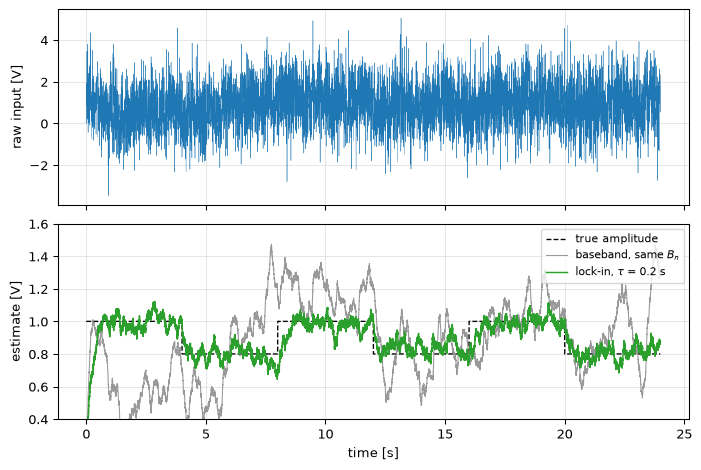
Figure 3: Tracking a hidden step. A 250 Hz carrier’s amplitude switches between 1.0 and 0.8 every 4 s (a 20% absorption change), buried in white + 1/f noise; the raw record (top, one trace, decimated for display) shows nothing usable. The streaming lock-in with τ = 0.2 s (bottom, green) recovers the staircase cleanly. Measuring the same quantity at baseband through an identical one-pole filter (gray) has the same noise bandwidth but sits on the 1/f mountain: it drifts by more than the step it is supposed to resolve.
per-state |error|: lock-in max 0.035 V, baseband max 0.239 V (step size 0.2 V)
The gray curve deserves a second look: it is not a straw man. It has the same filter, the same\(B_n\), the same everything except the carrier, and it is off by more than the step it should measure, in a direction and by an amount that change slowly and unpredictably. That is what “the noise is nonstationary at DC” does to an honest instrument, and no bandwidth choice fixes it.
The square-wave reference: a cheap trick and its exact price
Analogue lock-ins historically demodulated with a square reference, ±1, because a switch is easier to build than an accurate multiplier (and a digital implementation on a tiny MCU can do the same with additions only: see the embedded page). The square wave is the sum of the odd harmonics, \(\operatorname{sq}(\theta) = \tfrac{4}{\pi}(\cos\theta - \tfrac{1}{3}\cos 3\theta + \tfrac{1}{5}\cos 5\theta - \cdots)\), and each term does exactly what you would guess:
The fundamental demodulates the signal: after calibration by \(\pi/2\), a clean tone reads correctly.
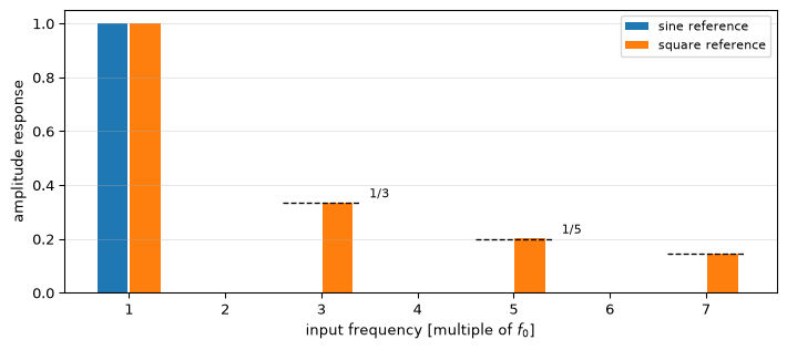
The harmonic terms demodulate other parts of the spectrum into your answer: input at \(3f_0\) appears at \(\tfrac{1}{3}\) weight, \(5f_0\) at \(\tfrac{1}{5}\), and so on. The lock-in stops being a single narrow window and becomes a comb of windows at every odd harmonic.
Against white noise, the harmonic windows collect noise but no signal, and the total penalty works out to exactly \(\pi^2/8\) in variance, about 0.9 dB: the sum \(1 + \tfrac{1}{9} + \tfrac{1}{25} + \cdots = \tfrac{\pi^2}{8}\) made audible.
Figure 4: What each reference hears (measured, 64 samples per carrier cycle). A sine reference responds at the carrier only. A square reference also responds at the odd harmonics with the predicted 1/3 and 1/5 weights, and its white-noise variance is π²/8 ≈ 1.23 times worse: the price of demodulating with a switch instead of a multiplier.
variance penalty: measured 1.191, pi^2/8 = 1.234
Digitally, the sine reference costs two table lookups per sample, so the square reference is no longer the default: use it only when even that is too much, and then place the carrier where the odd-harmonic windows land on quiet spectrum. Note that a square-wave excitation (an LED switched on/off, the practical choice) is entirely compatible with a sine demodulation: the excitation’s harmonics fall on the sine reference’s nulls, and only the fundamental, \(\tfrac{4}{\pi} \times \tfrac{1}{2}\) of the on/off depth, is measured. Bookkeeping, not distortion.
Choosing the carrier frequency
The bound \(\operatorname{var}(\hat{A}) = S(f_0)/T\) makes carrier choice almost mechanical. Three rules cover practice:
Above the corner, promptly. Every octave below \(f_c\) costs a factor of 2 in variance; above \(f_c\) the floor is flat and pushing higher buys essentially nothing. There is therefore no prize for heroic carrier frequencies: a corner at 20 Hz is escaped at a few hundred hertz. What pushing higher costs is front-end bandwidth (the photodiode amplifier of the embedded page rolls off, and its gain-bandwidth budget is spent on the carrier) and tighter timing.
Away from interference, by more than your bandwidth. The spectrum is not empty: mains hum sits in a comb at multiples of 50 Hz (or 60 Hz), switching converters and LED lighting add their own lines. The lock-in rejects an interferer offset \(\delta f\) from the carrier only by its filter’s stopband there: a block average responds as \(|\text{sinc}(\delta f\, T)|\), falling only as \(1/(\pi\,\delta f\, T)\), so a strong line near the carrier still hurts. Place \(f_0\) so the nearest expected line is many \(B_n\) away, and remember the square reference multiplies the places you must check by its harmonic comb.
On the coherent grid. Everything from the whole-cycles callout applies verbatim: an integration window spanning a non-integer number of carrier cycles leaks the negative-frequency image into the answer as a deterministic bias. Derive the carrier and the sample clock from the same source, and make \(f_0 = k f_s / N\) exact. On hardware this is a timer-configuration decision, made deliberately in the embedded companion.
The lock-in as a detector
The pages so far treat \(\hat{A}\) as an estimate. Often the actual question is a decision: is the tone there at all? Is the LED’s light reaching the photodiode, is the analyte present, did the contact close? That question has its own failure mode, and it is worth meeting here because the next page in this arc is about exactly this.
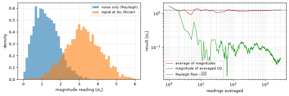
With no signal at all, the two demodulated quadratures are independent zero-mean Gaussians, so the magnitude\(\hat{A} = |z|\) is Rayleigh-distributed: strictly positive, with mean \(\sqrt{\pi/2}\,\sigma_z \approx 1.25\,\sigma_z\). A lock-in reading is therefore never zero, even with the input shorted, and averaging many magnitude readings converges confidently to that floor rather than to zero. The floor is not a bias in the instrument; it is what taking a magnitude does to noise.
Figure 5: Left: distribution of the lock-in magnitude with no signal present (Rayleigh, never zero, mean 1.25 σ_z) and with a signal at 3σ_z (Rician). The overlap is where detection errors live, and choosing the threshold is precisely the subject of detection theory. Right: with the input noise only, averaging successive magnitude readings converges to the Rayleigh floor (red), while averaging the complex I/Q outputs before taking the magnitude converges to zero (green): average first, rectify last.
mean noise-only magnitude: 1.256 sigma_z (Rayleigh mean sqrt(pi/2) = 1.253)
Two practical consequences. First, average I and Q, then take the magnitude, never the other way around; the right-hand plot is the entire argument. Second, deciding “signal present” means putting a threshold between those two overlapping histograms, and every placement trades misses against false alarms. That trade has a complete theory: thresholds, ROC curves, and the Neyman-Pearson lemma, previewed on the outlier-detection page and treated properly on the detection-theory page, which picks up these two histograms exactly where this section leaves them and turns them into closed-form false-alarm and detection probabilities.
From the archive: the front end that motivated this page
From the archive: a biosensor front end, 2007
This page’s sources include two of the author’s front-end design reviews from Philips Research (2007, 2008), for a magnetoresistive biosensor readout: magnetic beads over a GMR sensor, a wanted signal of nanovolt-per-root-hertz scale, and everything on this page visible in one slide. The problem statement plots the signal against the amplifier’s \(1/f\) noise and against crosstalk from the excitation sitting some 50 dB above it, with roughly 175 dB between the largest and smallest features on the axis; the solution moves the measurement up the spectrum and spends the dynamic-range budget on filtering before the ADC.
Two details from those decks resurface elsewhere in this workshop. The oversampling budget (trading analogue filter order against sample rate, “SQNR at 40 MHz lets a 2nd-order filter do a 4th-order job”) is the ADC-noise page’s oversampling argument, run in reverse. And one deliberately provocative line, “note that dithering is accomplished by interference”, is the dither page’s thesis wearing safety glasses: the interference the front end could not remove was at least randomising the quantiser. The 2008 deck’s charge-integrating photodiode front end reappears on the embedded page, where its \(kT/C\) noise bookkeeping is worked through.
On hardware
A lock-in is arguably the best measurement instrument a microcontroller can host: the DSP core is a multiply-accumulate against a table, the analogue demands are modest precisely because the method tolerates noise, and the result is a measurement that a naive design misses by orders of magnitude. The embedded companion builds an LED/photodiode photometer on both default platforms: carrier and sample clocks from one timer, a transimpedance front end sized by the formulas above, and a measured noise floor to compare against \(\sqrt{S(f_0)/T}\).
Going further
When the reference is not yours. This page assumes you generate the excitation, so frequency and phase are known exactly. When the carrier comes from elsewhere (a rotating chopper, the mains, a free-running oscillator) the reference must be recovered, by a phase-locked loop or by the frequency-estimation machinery of the previous page, and reference phase noise enters the error budget.
Averaging drift instead of escaping it. The wall in the averaging figure has a second, complementary treatment: characterise how the error grows with \(T\) instead of avoiding it. That is the Allan variance, the standard tool for oscillator and sensor drift, not covered here yet. Related strategies, chopper stabilisation and correlated double sampling, apply the modulation idea inside amplifiers and image sensors respectively: the trick of this page, miniaturised.
Weak signals with structure. The lock-in exploits one known parameter (frequency) to reject noise. The matched filter generalises to any known waveform; stochastic resonance shows that even noise itself can sometimes be recruited. And when the signal is a decision rather than a level, detection theory takes over where the Rayleigh floor above left off.
References
Emde, Gerhard von der. 1999. “Active Electrolocation of Objects in Weakly Electric Fish.”Journal of Experimental Biology 202 (10): 1205–15. https://doi.org/10.1242/jeb.202.10.1205.
Meade, Marcus L. 1983. Lock-in Amplifiers: Principles and Applications. London: Peter Peregrinus, on behalf of the Institution of Electrical Engineers.
Scofield, John H. 1994. “Frequency-Domain Description of a Lock-in Amplifier.”American Journal of Physics 62 (2): 129–33. https://doi.org/10.1119/1.17629.
---title: "Lock-in Detection"subtitle: "Measuring microvolts under a mountain of 1/f noise"description-meta: "Measuring microvolts under 1/f noise: modulate the quantity, demodulate synchronously, and move the measurement out of where the noise lives."bibliography: ../../references.bib---Some measurements are small and slow. The optical absorption of a blood sample, the resistance change of a strain gauge, the thermal signal of an infrared detector: quantities that change over seconds or not at all, buried in electronics whose noise grows without bound exactly where slow signals live. Averaging, the universal remedy of [estimation basics](../estimation-basics/index.qmd), quietly stops working there, and it does not warn you.The lock-in amplifier is the classic instrument built around the escape route [@meade1983lockin]: *move the measurement*. Modulate the physical quantity up to a carrier frequency where the front end is quiet, measure the carrier's amplitude, and you inherit the clean white-noise averaging law no matter what the noise does at DC. The [previous page](../estimating-a-sinusoid/index.qmd) already built the measuring device without saying so: the coherent single-bin DFT **is** the digital lock-in. This page is about the strategy wrapped around it: why 1/f noise forces you up in frequency, what integration time buys and at what bandwidth cost, and what it means to run one against real hardware ([the embedded companion](embedded.qmd) builds an LED photometer from it).::: {.callout-note title="Prerequisites"}Part of the [estimation & detection arc](../estimation-and-detection.qmd); the overview gives the reading order.[Estimating a sinusoid](../estimating-a-sinusoid/index.qmd) supplies the estimator this page reuses (the coherent single-bin DFT and its Cramér-Rao bound); [noise whitening](../noise-whitening/index.qmd) introduces $1/f^\alpha$ noise itself. [Noise and SNR](../../basics/03-noise-snr.qmd) and the modulation section of [convolution, correlation & modulation](../../basics/11-convolution-correlation-modulation.qmd) round out the background.:::::: {.callout-tip title="Code"}The implementation is [`lockin.py`](lockin.py). Save [`test_lockin.py`](test_lockin.py) beside it and `pytest test_lockin.py` runs the checks on it.:::```{python}#| echo: falseimport numpy as npimport matplotlib.pyplot as pltfrom scipy.signal import welchfrom lockin import (front_end_noise, lockin_block, lockin_stream, enbw, amplitude_noise_std)```<hr>## The enemy: a noise floor that is not flatEvery amplifier, every resistor, every ADC delivers a noise spectrum with the same general shape: a flat (white) floor at high frequencies, and a rise toward DC, usually close to $1/f$, from slow processes in the components themselves: carrier trapping in transistors, temperature drift, ageing [@ward20071f]. The two meet at the **corner frequency** $f_c$, anywhere from millihertz for a good instrumentation amplifier to kilohertz for a cheap op-amp. Throughout this page the noise model is$$S(f) = S_w\left(1 + \frac{f_c}{f}\right)$$with $S_w$ the one-sided white floor in $\text{V}^2/\text{Hz}$. Below $f_c$ the spectrum climbs without limit; a DC measurement sits at the bottom of that climb, at the worst point on the entire axis.```{python}#| label: fig-noise-floor#| fig-cap: "The front-end noise model, measured from a generated record (fs = 2 kHz, corner at 20 Hz) against the analytic S(f). A slow signal measured at baseband competes with the 1/f mountain; the same signal modulated to 250 Hz competes only with the white floor. The vertical distance between the two markers is the whole argument of this page."fs, sigma_w, corner =2000.0, 1.0, 20.0S_w =2* sigma_w**2/ fsrng = np.random.default_rng(42)x = front_end_noise(2**20, sigma_w, corner, fs=fs, rng=rng)f, P = welch(x, fs=fs, nperseg=8192)fig, ax = plt.subplots(figsize=(7.5, 3.8))ax.loglog(f[1:], P[1:], 'C0', lw=0.8, alpha=0.7, label='measured PSD (Welch)')ax.loglog(f[1:], S_w * (1+ corner / f[1:]), 'k--', lw=1.2, label=r'$S_w(1 + f_c/f)$')ax.axvline(corner, color='gray', ls=':', lw=1)ax.annotate('$f_c$', (corner, S_w *40), fontsize=10, ha='right')ax.plot([f[1]], [S_w * (1+ corner / f[1])], 'v', color='C3', ms=9, label='a DC measurement lives here')ax.plot([250], [S_w * (1+ corner /250)], '^', color='C2', ms=9, label='a modulated one lives here')ax.set_xlabel('frequency [Hz]'); ax.set_ylabel(r'PSD [V$^2$/Hz]')ax.legend(fontsize=8); ax.grid(True, which='both', alpha=0.3)fig.tight_layout(); plt.show()# The generator must actually deliver the calibrated S(f) the page# reasons with: check floor and 1/f region against the analytic curve.model = S_w * (1+ corner / f[1:])hi = f[1:] >500lo = (f[1:] >4) & (f[1:] <10)assertabs(np.mean(P[1:][hi] / model[hi]) -1) <0.05, "white floor off"assertabs(np.mean(P[1:][lo] / model[lo]) -1) <0.15, "1/f region off"```<hr>## Watching averaging failWhat does that mountain do to a measurement? Take the simplest possible task: estimate a constant level by averaging $T$ seconds of data. In white noise the answer is on [the estimation-basics page](../estimation-basics/index.qmd#consistency-and-why-averaging-buys-sqrtn): variance $\sigma^2/N$, so the error falls as $1/\sqrt{T}$, forever. In $1/f$ noise it does not.The mechanism is worth seeing without equations first. Averaging longer helps against noise that is *faster* than your averaging window, because fast wiggles cancel. But $1/f$ noise has ever more power at ever slower time scales: stretch the window and you admit new, slower drift that was invisible before. The two effects nearly cancel, and the error curve goes flat. More data stops buying accuracy: not slowly, not eventually, but at a wall a little past $1/f_c$ seconds.```{python}#| label: fig-averaging-wall#| fig-cap: "RMS error of a T-second average, measured over many disjoint blocks of one long record (fs = 2 kHz). In white noise (blue) the error falls as the promised T^(-1/2) across the whole sweep. In white + 1/f noise (red) the same estimator hits a wall near 1/f_c = 50 ms and a 300-fold increase in data buys almost nothing. The lock-in (green) measures the same record at a 250 Hz carrier instead, and recovers the white-noise law: its error keeps falling on the S(f0)/T line, three decades after the baseband curve has stopped."rng = np.random.default_rng(7)n_tot =2**21# ~17 minutes at 2 kHzxw = sigma_w * rng.standard_normal(n_tot)xp = front_end_noise(n_tot, sigma_w, corner, fs=fs, rng=rng)Ts = np.array([0.032, 0.1, 0.32, 1.0, 3.2, 10.0])f0 =250.0rms_w, rms_p, rms_l = [], [], []for T in Ts: nblk =int(round(T * fs)) nb =min(n_tot // nblk, 96) blk =lambda x: x[:nb * nblk].reshape(nb, nblk) rms_w.append(np.sqrt(np.mean(blk(xw).mean(axis=1)**2))) rms_p.append(np.sqrt(np.mean(blk(xp).mean(axis=1)**2)))# Lock-in: a unit-amplitude carrier on an exact bin of each block,# demodulated per block; the error is the amplitude misread. k =round(f0 * nblk / fs) f0b = k * fs / nblk tone = np.cos(2* np.pi * f0b * np.arange(nblk) / fs +0.3) errs = [lockin_block(seg + tone, f0b, fs=fs)[0] -1.0for seg in blk(xp)] rms_l.append(np.sqrt(np.mean(np.square(errs))))rms_w, rms_p, rms_l =map(np.array, (rms_w, rms_p, rms_l))S1_f0 = S_w * (1+ corner / f0)fig, ax = plt.subplots(figsize=(7.5, 4))ax.loglog(Ts, rms_w, 'o-C0', ms=4, label='baseband average, white noise')ax.loglog(Ts, rms_p, 's-C3', ms=4, label='baseband average, white + 1/f')ax.loglog(Ts, rms_l, '^-C2', ms=4, label='lock-in at 250 Hz, same 1/f record')ax.loglog(Ts, np.sqrt(S_w / (2* Ts)), 'C0:', lw=1, label=r'$\sqrt{S_w/2T}$')ax.loglog(Ts, np.sqrt(S1_f0 / Ts), 'C2:', lw=1, label=r'$\sqrt{S(f_0)/T}$')ax.set_xlabel('integration time T [s]'); ax.set_ylabel('RMS error [V]')ax.legend(fontsize=8); ax.grid(True, which='both', alpha=0.3)fig.tight_layout(); plt.show()gain_w = rms_w[0] / rms_w[-1]gain_p = rms_p[0] / rms_p[-1]gain_l = rms_l[0] / rms_l[-1]print(f"312x more data: white baseband {gain_w:.1f}x better, "f"1/f baseband {gain_p:.1f}x, lock-in {gain_l:.1f}x "f"(sqrt(312) = {np.sqrt(Ts[-1]/Ts[0]):.1f})")# White baseband must sit on sqrt(S_w/2T) throughout (the DC-level# bound has a factor 2: see the callout below).assert np.all(np.abs(rms_w / np.sqrt(S_w / (2* Ts)) -1) <0.2)# The wall: 1/f baseband improves by far less than sqrt(312) = 17.7.assert gain_p <3.0, "1/f averaging should hit a wall"assert gain_w >12.0, "white averaging should not"# The lock-in recovers the white law ON THE SAME 1/f RECORD.assert np.all((rms_l / np.sqrt(S1_f0 / Ts) >0.75)& (rms_l / np.sqrt(S1_f0 / Ts) <1.3))assert gain_l >12.0, "the lock-in should keep improving"```This is the plot that justifies everything else here. The red curve is not a badly built estimator; it is the *best linear* estimator for the job it was given, and the job is unwinnable. The green curve is the same record, the same total data, with the measurement moved 250 Hz up the spectrum first.<hr>## The fix: modulate up, demodulate downSo the strategy is: make the physical quantity ride a carrier. Chop the light with the LED drive, excite the bridge with an AC reference, vibrate the sample. If the measurand is $m$ and the excitation is a carrier at $f_0$, the front end now delivers$$x(t) = \underbrace{G\, m \cos(2\pi f_0 t + \phi)}_{\text{signal, parked at } f_0} + \; w(t)$$and estimating $m$ means estimating the **amplitude of a tone of known frequency**, which is a solved problem: the coherent single-bin DFT from [the previous page](../estimating-a-sinusoid/index.qmd#known-frequency-the-coherent-single-bin-dft), which correlates the record with quadrature references at $f_0$ and reads amplitude and phase off the complex result. A lock-in amplifier is that inner product, plus the modulation strategy, plus a low-pass filter to let you watch the amplitude move. `lockin_block` in this topic's module is `coherent_dft` with a different hat on; the [Goertzel filter](../goertzel/index.qmd) is the same inner product computed recursively.::: {.callout-tip title="Nature's version of carrying your own carrier" appearance="simple"}Supplying your own excitation so the measurement lands where you want it is a sensing strategy weakly electric fish arrived at first. The fish continuously emits an electric organ discharge, and nearby objects change the discharge-driven current at electroreceptors in its skin according to their conductivity, so what the receptors read is a **modulation of the animal's own transmitted carrier** rather than any field the environment happened to provide [@vonderemde1999active]. The same fish appears on the [adaptive-filtering](../adaptive-filtering/index.qmd) page for a different trick entirely: shifting its carrier frequency away from a neighbour's, which is the interference half of the same design problem.Keep the claim narrow. Nothing here says the fish demodulates coherently or multiplies by a reference; its electroreceptors are tuned analogue sensors, and the paper describes electric images on the skin, not a phase-sensitive detector. What carries over is the architectural choice that opens this section: *generate the carrier yourself*, and a hard sensing problem becomes the measurement of a modulation at a frequency you control and know exactly. The photometer on [the embedded page](embedded.qmd) makes the same choice with an LED.:::What did moving to $f_0$ buy, exactly? For noise that is (locally) white around the carrier, the amplitude estimate from $T$ seconds obeys$$\operatorname{var}(\hat{A}) = \frac{S(f_0)}{T}$$and this is not merely what the single-bin DFT achieves, it is the Cramér-Rao bound: no estimator does better. The noise that matters is evaluated **at the carrier**, where the front end is quiet, and the $1/f$ mountain at DC never appears in the formula. That substitution, $S(0^+) \to S(f_0)$, is the entire value of the instrument.::: {.callout-warning title="Bounds get checked here: the exact Fisher matrix, again"}The [previous page](../estimating-a-sinusoid/index.qmd#unknown-frequency-the-1n3-law) earned a scar proving closed-form bounds wrong from memory, and this one is quoted for *colored* noise, where hand-waving is even easier. So it gets the same treatment: build the exact Fisher information matrix, numerically, with the true noise covariance, and compare. For AR(1) noise, whose covariance and spectrum are both known exactly, the demo below finds $S(f_0)/T$ within a fraction of a percent of the exact bound, and `test_colored_noise_bound_is_psd_at_f0_over_T` pins it permanently. The requirement is only that $S(f)$ is flat *across the lock-in's own bandwidth* around $f_0$ (a few $1/T$), which is exactly what modulating above the corner arranges.:::```{python}#| label: fisher-check# The page's central formula, against the exact Fisher information for# AR(1) noise: x[n] = A cos(2 pi f0 n + phi) + v[n], v[n] = a v[n-1] + e[n].from scipy.linalg import toeplitzN =512for a_coef, f0n in [(0.9, 0.25), (0.9, 0.10), (0.5, 0.20)]: acf = a_coef**np.arange(N) / (1- a_coef**2) # unit innovations Ci = np.linalg.inv(toeplitz(acf)) psi =2* np.pi * f0n * np.arange(N) +0.7 G = np.vstack([np.cos(psi), -np.sin(psi)]) # d/dA, d/dphi at A=1 exact = np.linalg.inv(G @ Ci @ G.T)[0, 0] S1 =2/ np.abs(1- a_coef * np.exp(-2j* np.pi * f0n))**2 closed = S1 / N # S(f0)/T at fs = 1print(f"AR(1) a={a_coef}, f0={f0n:.2f}: exact {exact:.5e}, "f"S(f0)/T {closed:.5e}, ratio {exact / closed:.4f}")assertabs(exact / closed -1) <0.01, "closed form must match the FIM"```::: {.callout-note title="The honest fine print: a factor of 2, and where it went"}Compare the two dotted reference lines in the averaging figure. The baseband average in white noise follows $\sqrt{S_w/2T}$; the lock-in follows $\sqrt{S(f_0)/T}$, twice the variance at the same $T$. That factor is real and structural: a DC level uses every sample at full weight, while an amplitude rides a cosine whose mean square is $\tfrac{1}{2}$, so half the record's leverage is gone (the same $\tfrac{1}{2}$ that haunted [the SNR parameterisation trap](../estimating-a-sinusoid/index.qmd#unknown-frequency-the-1n3-law)). Modulation costs 3 dB against a *hypothetical drift-free* DC measurement, and buys back orders of magnitude against the real one. Textbook treatments often skip this admission; measure it and it is exactly there.:::<hr>## Bandwidth: what the low-pass filter is really choosingThe block average above answers "what was the amplitude over these $T$ seconds". A real instrument more often wants to *watch* the amplitude: track the absorption as the sample flows past, follow the strain as the load changes. The streaming form replaces "average the whole block" with a low-pass filter on the demodulated quadratures, classically one-pole with time constant $\tau$ (the big knob on every analogue lock-in's front panel [@scofield1994frequency]).Every choice of filter is a choice of **equivalent noise bandwidth** $B_n$: the width of the ideal brick-wall filter that would pass the same noise power. The variance rule generalises to$$\operatorname{var}(\hat{A}) = 2\, S(f_0)\, B_n, \qquad B_n = \frac{1}{2T} \text{ (block average)}, \quad B_n = \frac{1}{4\tau} \text{ (one-pole)}$$(the factor 2 folds both sidebands of the carrier onto the output; with $B_n = 1/2T$ it reproduces $S(f_0)/T$ exactly). The trade is stated in one line: **noise floor $\propto \sqrt{B_n}$, and $B_n$ is the fastest signal change you can follow.** A lock-in with $\tau = 1$ s has $B_n = 0.25$ Hz: it rejects everything the spectrum holds except a quarter-hertz sliver around the carrier, and correspondingly cannot see your signal change faster than seconds. Narrowband rejection and sluggishness are the same purchase.```{python}#| label: fig-tracking#| fig-cap: "Tracking a hidden step. A 250 Hz carrier's amplitude switches between 1.0 and 0.8 every 4 s (a 20% absorption change), buried in white + 1/f noise; the raw record (top, one trace, decimated for display) shows nothing usable. The streaming lock-in with τ = 0.2 s (bottom, green) recovers the staircase cleanly. Measuring the same quantity at baseband through an identical one-pole filter (gray) has the same noise bandwidth but sits on the 1/f mountain: it drifts by more than the step it is supposed to resolve."rng = np.random.default_rng(19)dur, f0, tau =24.0, 250.0, 0.2n =int(dur * fs)t = np.arange(n) / fslevel = np.where((t //4).astype(int) %2==0, 1.0, 0.8)noise = front_end_noise(n, sigma_w, corner, fs=fs, rng=rng)x_mod = level * np.cos(2* np.pi * f0 * t) + noise # modulated front endx_base = level + noise # baseband front endr, _ = lockin_stream(x_mod, f0, fs=fs, tau=tau)b = np.exp(-1/ (fs * tau))from scipy.signal import lfilterbase = lfilter([1- b], [1, -b], x_base)fig, axes = plt.subplots(2, 1, figsize=(7.5, 5), sharex=True)axes[0].plot(t[::8], x_mod[::8], 'C0', lw=0.3)axes[0].set_ylabel('raw input [V]')axes[0].grid(True, alpha=0.3)axes[1].plot(t, level, 'k--', lw=1, label='true amplitude')axes[1].plot(t, base, color='gray', lw=0.8, alpha=0.8, label='baseband, same $B_n$')axes[1].plot(t, r, 'C2', lw=1.1, label=r'lock-in, $\tau$ = 0.2 s')axes[1].set_xlabel('time [s]'); axes[1].set_ylabel('estimate [V]')axes[1].set_ylim(0.4, 1.6); axes[1].legend(fontsize=8, loc='upper right')axes[1].grid(True, alpha=0.3)fig.tight_layout(); plt.show()# Settled windows: the second half of each 4 s state, skipping the first.err_lock, err_base = [], []for k inrange(1, 6): sl =slice(int((4* k +2) * fs), int((4* k +4) * fs)) truth = level[sl].mean() err_lock.append(r[sl].mean() - truth) err_base.append(base[sl].mean() - truth)err_lock, err_base = np.abs(err_lock), np.abs(err_base)print(f"per-state |error|: lock-in max {err_lock.max():.3f} V, "f"baseband max {err_base.max():.3f} V (step size 0.2 V)")# The lock-in must resolve the 0.2 V step comfortably; the baseband# chain, with the SAME noise bandwidth, must drift by more than the# step itself, which is exactly what the caption claims.assert err_lock.max() <0.05, "lock-in should recover each level"assert err_base.max() >0.2, "baseband drift should exceed the 0.2 V step"```The gray curve deserves a second look: it is not a straw man. It has the *same* filter, the *same* $B_n$, the same everything except the carrier, and it is off by more than the step it should measure, in a direction and by an amount that change slowly and unpredictably. That is what "the noise is nonstationary at DC" does to an honest instrument, and no bandwidth choice fixes it.<hr>## The square-wave reference: a cheap trick and its exact priceAnalogue lock-ins historically demodulated with a **square** reference, ±1, because a switch is easier to build than an accurate multiplier (and a digital implementation on a tiny MCU can do the same with additions only: see [the embedded page](embedded.qmd)). The square wave is the sum of the odd harmonics, $\operatorname{sq}(\theta) = \tfrac{4}{\pi}(\cos\theta - \tfrac{1}{3}\cos 3\theta + \tfrac{1}{5}\cos 5\theta - \cdots)$, and each term does exactly what you would guess:- The fundamental demodulates the signal: after calibration by $\pi/2$, a clean tone reads correctly.- The harmonic terms demodulate *other parts of the spectrum into your answer*: input at $3f_0$ appears at $\tfrac{1}{3}$ weight, $5f_0$ at $\tfrac{1}{5}$, and so on. The lock-in stops being a single narrow window and becomes a comb of windows at every odd harmonic.- Against white noise, the harmonic windows collect noise but no signal, and the total penalty works out to exactly $\pi^2/8$ in variance, about 0.9 dB: the sum $1 + \tfrac{1}{9} + \tfrac{1}{25} + \cdots = \tfrac{\pi^2}{8}$ made audible.```{python}#| label: fig-square-reference#| fig-cap: "What each reference hears (measured, 64 samples per carrier cycle). A sine reference responds at the carrier only. A square reference also responds at the odd harmonics with the predicted 1/3 and 1/5 weights, and its white-noise variance is π²/8 ≈ 1.23 times worse: the price of demodulating with a switch instead of a multiplier."n_h = np.arange(64*400)f0n =1.0/64ks = np.arange(1, 8)resp_sin, resp_sq = [], []for k in ks: xk = np.cos(2* np.pi * k * f0n * n_h +1.1) resp_sin.append(lockin_block(xk, f0n)[0]) resp_sq.append(lockin_block(xk, f0n, reference='square')[0])fig, ax = plt.subplots(figsize=(7.5, 3.4))ax.bar(ks -0.17, resp_sin, 0.32, label='sine reference')ax.bar(ks +0.17, resp_sq, 0.32, label='square reference')for k in (3, 5, 7): ax.plot([k -0.4, k +0.4], [1/ k] *2, 'k--', lw=1)ax.text(3.5, 1/3+0.02, '1/3', fontsize=8)ax.text(5.5, 1/5+0.02, '1/5', fontsize=8)ax.set_xlabel('input frequency [multiple of $f_0$]')ax.set_ylabel('amplitude response')ax.legend(fontsize=8); ax.grid(True, axis='y', alpha=0.3)fig.tight_layout(); plt.show()# Measured variance penalty vs the pi^2/8 prediction.rng = np.random.default_rng(5)Nv =4096f0v =256/ Nvtone = np.cos(2* np.pi * f0v * np.arange(Nv) +0.7)a_sin, a_sq = [], []for _ inrange(2000): xv = tone + rng.standard_normal(Nv) a_sin.append(lockin_block(xv, f0v)[0]) a_sq.append(lockin_block(xv, f0v, reference='square')[0])ratio = np.var(a_sq) / np.var(a_sin)print(f"variance penalty: measured {ratio:.3f}, pi^2/8 = {np.pi**2/8:.3f}")assertabs(resp_sq[2] -1/3) <0.02andabs(resp_sq[4] -1/5) <0.02assertmax(resp_sq[1], resp_sq[3]) <1e-6, "even harmonics rejected"assertmax(resp_sin[1:]) <1e-10, "sine hears the carrier only"assertabs(ratio / (np.pi**2/8) -1) <0.10```Digitally, the sine reference costs two table lookups per sample, so the square reference is no longer the default: use it only when even that is too much, and then place the carrier where the odd-harmonic windows land on quiet spectrum. Note that a square-wave *excitation* (an LED switched on/off, the practical choice) is entirely compatible with a sine *demodulation*: the excitation's harmonics fall on the sine reference's nulls, and only the fundamental, $\tfrac{4}{\pi} \times \tfrac{1}{2}$ of the on/off depth, is measured. Bookkeeping, not distortion.<hr>## Choosing the carrier frequencyThe bound $\operatorname{var}(\hat{A}) = S(f_0)/T$ makes carrier choice almost mechanical. Three rules cover practice:**Above the corner, promptly.** Every octave below $f_c$ costs a factor of 2 in variance; above $f_c$ the floor is flat and pushing higher buys essentially nothing. There is therefore no prize for heroic carrier frequencies: a corner at 20 Hz is escaped at a few hundred hertz. What pushing higher *costs* is front-end bandwidth (the photodiode amplifier of [the embedded page](embedded.qmd) rolls off, and its gain-bandwidth budget is spent on the carrier) and tighter timing.**Away from interference, by more than your bandwidth.** The spectrum is not empty: mains hum sits in a comb at multiples of 50 Hz (or 60 Hz), switching converters and LED lighting add their own lines. The lock-in rejects an interferer offset $\delta f$ from the carrier only by its filter's stopband there: a block average responds as $|\text{sinc}(\delta f\, T)|$, falling only as $1/(\pi\,\delta f\, T)$, so a strong line *near* the carrier still hurts. Place $f_0$ so the nearest expected line is many $B_n$ away, and remember the square reference multiplies the places you must check by its harmonic comb.**On the coherent grid.** Everything from the [whole-cycles callout](../estimating-a-sinusoid/index.qmd#known-frequency-the-coherent-single-bin-dft) applies verbatim: an integration window spanning a non-integer number of carrier cycles leaks the negative-frequency image into the answer as a deterministic bias. Derive the carrier and the sample clock from the same source, and make $f_0 = k f_s / N$ exact. On hardware this is a timer-configuration decision, made deliberately in [the embedded companion](embedded.qmd).<hr>## The lock-in as a detectorThe pages so far treat $\hat{A}$ as an *estimate*. Often the actual question is a decision: is the tone there at all? Is the LED's light reaching the photodiode, is the analyte present, did the contact close? That question has its own failure mode, and it is worth meeting here because the next page in this arc is about exactly this.With no signal at all, the two demodulated quadratures are independent zero-mean Gaussians, so the *magnitude* $\hat{A} = |z|$ is *Rayleigh*-distributed: strictly positive, with mean $\sqrt{\pi/2}\,\sigma_z \approx 1.25\,\sigma_z$. A lock-in reading is therefore **never zero**, even with the input shorted, and averaging many magnitude readings converges confidently to that floor rather than to zero. The floor is not a bias in the instrument; it is what taking a magnitude does to noise.```{python}#| label: fig-detector#| fig-cap: "Left: distribution of the lock-in magnitude with no signal present (Rayleigh, never zero, mean 1.25 σ_z) and with a signal at 3σ_z (Rician). The overlap is where detection errors live, and choosing the threshold is precisely the subject of detection theory. Right: with the input noise only, averaging successive magnitude readings converges to the Rayleigh floor (red), while averaging the complex I/Q outputs before taking the magnitude converges to zero (green): average first, rectify last."rng = np.random.default_rng(11)Nd =1024f0d =64/ Ndtheta =2* np.pi * f0d * np.arange(Nd)sigma_z = np.sqrt(2*1.0**2/ Nd) # per-quadrature std, sigma=1mags0, zs0, mags1 = [], [], []for _ inrange(3000): w = rng.standard_normal(Nd) z0 =2* np.mean(w * np.exp(-1j* theta)) z1 =2* np.mean((w +3* sigma_z * np.cos(theta +0.5))* np.exp(-1j* theta)) mags0.append(np.abs(z0)); zs0.append(z0); mags1.append(np.abs(z1))mags0, mags1 = np.array(mags0), np.array(mags1)zs0 = np.array(zs0)fig, axes = plt.subplots(1, 2, figsize=(10, 3.4))bins = np.linspace(0, 6* sigma_z, 50)axes[0].hist(mags0 / sigma_z, bins=bins / sigma_z, density=True, alpha=0.6, label='noise only (Rayleigh)')axes[0].hist(mags1 / sigma_z, bins=bins / sigma_z, density=True, alpha=0.6, label=r'signal at $3\sigma_z$ (Rician)')axes[0].set_xlabel(r'magnitude reading [$\sigma_z$]')axes[0].set_ylabel('density'); axes[0].legend(fontsize=8)axes[0].grid(True, alpha=0.3)n_avg = np.arange(1, len(mags0) +1)axes[1].loglog(n_avg, np.abs(np.cumsum(mags0) / n_avg) / sigma_z, 'C3', lw=1, label='average of magnitudes')axes[1].loglog(n_avg, np.abs(np.cumsum(zs0) / n_avg) / sigma_z, 'C2', lw=1, label='magnitude of averaged I/Q')axes[1].axhline(np.sqrt(np.pi /2), color='k', ls='--', lw=0.8, label=r'Rayleigh floor $\sqrt{\pi/2}$')axes[1].set_xlabel('readings averaged')axes[1].set_ylabel(r'result [$\sigma_z$]')axes[1].legend(fontsize=8); axes[1].grid(True, which='both', alpha=0.3)fig.tight_layout(); plt.show()floor = np.sqrt(np.pi /2) * sigma_zprint(f"mean noise-only magnitude: {mags0.mean() / sigma_z:.3f} sigma_z "f"(Rayleigh mean sqrt(pi/2) = {np.sqrt(np.pi /2):.3f})")assertabs(mags0.mean() / floor -1) <0.05, "the Rayleigh floor is real"assert np.abs(zs0.mean()) < floor /10, "averaging I/Q first removes it"```Two practical consequences. First, **average I and Q, then take the magnitude**, never the other way around; the right-hand plot is the entire argument. Second, deciding "signal present" means putting a threshold between those two overlapping histograms, and every placement trades misses against false alarms. That trade has a complete theory: thresholds, ROC curves, and the Neyman-Pearson lemma, previewed on [the outlier-detection page](../outlier-detection/index.qmd#which-detector-at-which-threshold-the-roc-curve) and treated properly on [the detection-theory page](../detection-theory/index.qmd#the-lock-in-as-a-detector-finished), which picks up these two histograms exactly where this section leaves them and turns them into closed-form false-alarm and detection probabilities.<hr>## From the archive: the front end that motivated this page::: {.callout-note title="From the archive: a biosensor front end, 2007"}This page's sources include two of the author's front-end design reviews from Philips Research (2007, 2008), for a magnetoresistive biosensor readout: magnetic beads over a GMR sensor, a wanted signal of nanovolt-per-root-hertz scale, and everything on this page visible in one slide. The problem statement plots the signal against the amplifier's $1/f$ noise and against crosstalk from the excitation sitting some 50 dB above it, with roughly 175 dB between the largest and smallest features on the axis; the solution moves the measurement up the spectrum and spends the dynamic-range budget on filtering *before* the ADC.Two details from those decks resurface elsewhere in this workshop. The oversampling budget (trading analogue filter order against sample rate, "SQNR at 40 MHz lets a 2nd-order filter do a 4th-order job") is the [ADC-noise page's](../adc-noise/index.qmd) oversampling argument, run in reverse. And one deliberately provocative line, *"note that dithering is accomplished by interference"*, is the [dither page's](../dither/index.qmd) thesis wearing safety glasses: the interference the front end could not remove was at least randomising the quantiser. The 2008 deck's charge-integrating photodiode front end reappears on [the embedded page](embedded.qmd), where its $kT/C$ noise bookkeeping is worked through.:::<hr>## On hardwareA lock-in is arguably the best measurement instrument a microcontroller can host: the DSP core is a multiply-accumulate against a table, the analogue demands are modest precisely *because* the method tolerates noise, and the result is a measurement that a naive design misses by orders of magnitude. [The embedded companion](embedded.qmd) builds an LED/photodiode photometer on both default platforms: carrier and sample clocks from one timer, a transimpedance front end sized by the formulas above, and a measured noise floor to compare against $\sqrt{S(f_0)/T}$.<hr>## Going further**When the reference is not yours.** This page assumes you generate the excitation, so frequency and phase are known exactly. When the carrier comes from elsewhere (a rotating chopper, the mains, a free-running oscillator) the reference must be *recovered*, by a phase-locked loop or by the [frequency-estimation machinery](../estimating-a-sinusoid/index.qmd#estimators-from-the-bin-grid-to-the-bound) of the previous page, and reference phase noise enters the error budget.**Averaging drift instead of escaping it.** The wall in the averaging figure has a second, complementary treatment: characterise *how* the error grows with $T$ instead of avoiding it. That is the Allan variance, the standard tool for oscillator and sensor drift, not covered here yet. Related strategies, chopper stabilisation and correlated double sampling, apply the modulation idea *inside* amplifiers and image sensors respectively: the trick of this page, miniaturised.**Weak signals with structure.** The lock-in exploits one known parameter (frequency) to reject noise. The [matched filter](../matched-filtering/index.qmd) generalises to any known waveform; [stochastic resonance](../stochastic-resonance/index.qmd) shows that even noise itself can sometimes be recruited. And when the signal is a *decision* rather than a level, [detection theory](../detection-theory/index.qmd) takes over where the Rayleigh floor above left off.## References::: {#refs}:::